Regression corrected

If you read my post about regression from yesterday, you may have noticed that it has a serious problem with the way the errors were generated. What I did was this:

set.seed(157) x = runif(10) e = x for (i in 1:length(x)) { e[i] = rnorm(1,mean=x[i],sd=0.3) } y = 2.4*x + e plot(y~x,pch=16,col='blue',cex=1.8)

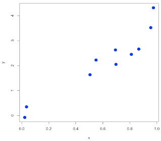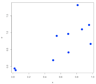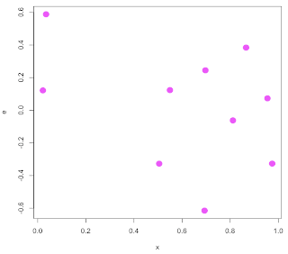
If we look at the errors, we see that they are dependent on the value of x! Naturally (b/c of mean=x[i]).

plot(x,e,pch=16,col='blue',cex=2)

What I should have done is something like this:

set.seed(1357) e = rnorm(10)/3 y = 2.4*x + e plot(x,e,pch=16,col='magenta',cex=2)

plot(x,y,pch=16,col='darkred',cex=2)

Nevertheless, I hope the essential points are clear:

• covariance is related to variance: cov(x,x) = var(x)
• correlation is the covariance of z-scores
• the slope of the regression line is: cov(x,y) / var(x)
• the regression line goes through x, y
• r ≈ cov(x,y) / sqrt(var(x)*var(y))
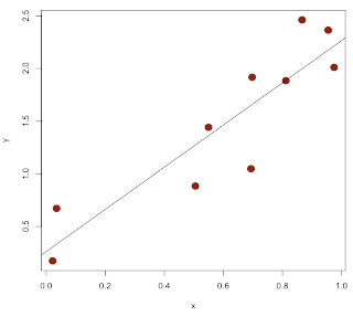
• the call to plot the line is abline(lm(y~x))

The proportionality for r is b/c we are not matching R's output for this. I think it is because we are missing a correction factor of n-1/n. I will have to look into that when I get back to my library at home.

With the change, we do a little better on guessing the slope:

> lm(y~x) Call: lm(formula = y ~ x) Coefficients: (Intercept) x 0.2625 2.0039