Basic regression

Continuing with my education in statistics, I'm reading Dalgaard's book, Introductory Statistics with R. The topic of this post is linear regression by least squares.

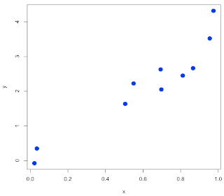
We're going to model errors in the data as follows:

set.seed(157) x = runif(10) e = x for (i in 1:length(x)) { e[i] = rnorm(1,mean=x[i],sd=0.3) } y = 2.4*x + e plot(y~x,pch=16,col='blue',cex=1.8)

[UPDATE: this is not the correct way to model the errors. See here.]

dx = x-mean(x) dy = y-mean(y) n = length(x) sum(dx**2)/(n-1) var(x)

The variance of x is computed in the usual way:

> sum(dx**2)/(n-1) [1] 0.1182592 > var(x) [1] 0.1182592

The covariance of x and y is defined in such a way that the variance of x is equal to the covariance of x with itself. That makes it easy to remember!

sum(dx*dy)/(n-1) cov(x,y)

> sum(dx*dy)/(n-1) [1] 0.4309724 > cov(x,y) [1] 0.4309724

Correlation is just like covariance, only it is computed using z-scores (normalized data).

zx = (x-mean(x))/sd(x) zy = (y-mean(y))/sd(y) cov(zx,zy) cor(x,y)

> cov(zx,zy) [1] 0.9515839 > cor(x,y) [1] 0.9515839

As discussed in Dalgard (Ch. 5), the estimated slope is:

β = cov(x,y) / var(x)

> cov(x,y) / var(x) [1] 3.644302

while the intercept is:

α = y - β*x

The linear regression line goes through x, y.

Let R do the work:

> lm(y~x) Call: lm(formula = y ~ x) Coefficients: (Intercept) x -0.04804 3.64430

The estimated slope is 3.64, while the true value is 2.4. I thought the problem was the last point, but it goes deeper than that.

># doing this by hand > i = 7 # index of max y value > lm(y[-i]~x[-i]) Call: lm(formula = y[-i] ~ x[-i]) Coefficients: (Intercept) x[-i] -0.1053 3.5803

Much more information is available using the "extractor function" summary:

> summary(xy.model) Call: lm(formula = y ~ x) Residuals: Min 1Q Median 3Q -0.456059 -0.369435 -0.006057 0.239960 Max 0.814548 Coefficients: Estimate Std. Error t value (Intercept) -0.04804 0.28819 -0.167 x 3.64430 0.41621 8.756 Pr(>|t|) (Intercept) 0.872 x 2.27e-05 *** --- Signif. codes: 0 ‘***’ 0.001 ‘**’ 0.01 ‘*’ 0.05 ‘.’ 0.1 ‘ ’ 1 Residual standard error: 0.4294 on 8 degrees of freedom Multiple R-squared: 0.9055, Adjusted R-squared: 0.8937 F-statistic: 76.67 on 1 and 8 DF, p-value: 2.267e-05

The correlation coefficient is

r = sum(dx*dy) / sqrt( sum(dx**2) * sum(dy**2) )

That is

r = cov(x,y) / sqrt(var(x)*var(y))

> cov(x,y) / sqrt(var(x)*var(y)) [1] 0.9515839

I am not sure why this doesn't match the output above.

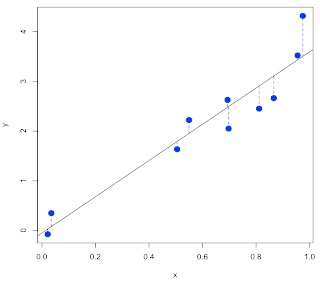
To get the plot shown at the top of the post we use another extractor function on the linear model:

xy.model = lm(y~x) w = fitted(xy.model)

w contains the predicted values of y for each x according to the model.

plot(y~x,pch=16,col='blue',cex=1.8) xy.model = lm(y~x) abline(xy.model) segments(x,w,x,y,col='blue',lty=2)

We can do an even fancier plot, with confidence bands, as follows.

df = data.frame(x) pp = predict(xy.model,int='p',newdata=df) pc = predict(xy.model,int='c',newdata=df) plot(y~x,pch=16,col='blue',cex=1.8) matlines(x,pc,lty=2,col='black') matlines(x,pp,lty=3,col='black')

This is promising but it is obviously going to take more work.