Testing

It seems improbable, but it is a fact that on the first exam in some courses, a few students may score lower than expected for guessing at random. We usually see some scores of less than 20 out of 100 for an exam whose questions have five possible answers ABCDE.

We can turn this into an illustration of statistical significance. How high must a score be before one can dismiss the null hypothesis (no knowledge of the subject) with a p-value of 0.05?

We have a Bernouli trial with p = 0.2.

The expected value or mean is np. There is a beautifully simple derivation of the mean and variance in the wikipedia article, the variance is np(1-p). For our example, the mean is 20 and the variance is 100 x 0.2 x 0.8, so the standard deviation is √16 = 4.

For a large class (N = 100) of randomly answering students, the distribution appraches normal, and we expect that 2.5% of such students will score at or above two standard deviations above the mean. To make our rate for a type I error less than 0.05, we should require a score of 28 or higher.

I wrote a short script to simulate this. Each student takes a test with 100 questions, and each trial consists of a class of 100 students. We count the number of students with scores at or above a threshold T. The results for 10 trials are printed, and the results for 100 trials are averaged.

A few quick points: the mean appears to fall between 20 and 21. I'm sure there's a simple explanation but it eludes me at the moment. The score that 2.5% of students regularly exceed is 28.

This is a great example of the danger of multiple hypothesis testing!

One last thing is that the code is not very smart. What I should have done was extract the statistics for each value of T for each trial, rather than repeating the trial for each value of T. But it runs fast enough, and this way I don't need a data structure to remember the results.

> python script.py 20: 56 43 54 57 57 54 57 46 45 64 55.0 21: 39 48 42 44 39 44 48 48 50 48 43.5 22: 43 32 39 30 38 35 36 42 33 41 34.6 23: 40 29 35 31 27 19 30 20 31 25 26.0 24: 19 18 24 26 20 22 21 17 15 24 19.2 25: 11 14 8 8 13 11 12 15 17 13 12.9 26: 12 6 6 6 11 4 8 7 10 6 9.2 27: 7 4 6 5 8 7 5 7 7 7 5.9 28: 3 2 4 2 3 1 2 3 5 1 3.6 29: 4 4 2 2 2 1 3 1 0 1 2.2 30: 1 1 1 0 1 1 1 0 0 1 0.9 31: 4 0 1 0 0 0 0 0 0 0 0.6 32: 0 0 0 0 1 0 0 1 0 0 0.3 33: 0 0 0 0 0 1 0 0 0 1 0.1 34: 0 0 0 0 0 0 0 0 1 0 0.1

script.py

import random def student(N=100, p=0.2): L = [random.random() <= p for i in range(N)] return sum(L) def trial(T): L = [student() for i in range(100)] return sum([1 for n in L if n >= T]) def mean(L): return 1.0*sum(L)/len(L) for T in range(20,35): L = list() print '%2d: ' % T, for i in range(100): L.append(trial(T)) if i < 10: print '%2d' % L[-1], print '%4.1f' % mean(L)

e again

I came across a neat quote from Martin Gardner:

The number e is as ubiquitous as pi, turning up everywhere, and especially in probability theory. If you randomly select real numbers between 0 and 1, and continue until their sum exceeds 1, the expected number of choices is e.

-Martin Gardner
note in Calculus Made Easy, p. 153

Of course, this begs for a Python simulation:

import random def mean(L): return float(sum(L))/len(L) def oneTrial(): counter = 1 f = random.random() while f <= 1: counter +=1 f += random.random() return counter N = int(1E7) L = [oneTrial() for i in range(N)] print mean(L)

> python script.py 2.7183671

A derivation would be nice, but that'll have to wait. I wonder about the variance.

nothing in biology makes sense except in the light of evolution

I've been reading Mike Yarus's book: Life from an RNA world (Amazon). It's a very readable account of evolution from the perspective of sequences and the RNA world. Mike's a highly intelligent guy, and that and his wit inform every page. In one chapter, he gets Rob Knight and Steve Freeland to do an evolution simulation.

we let a computer write out a random string, mutate 1 in 100 characters in each generation, and select changes only if they match Dobzhansky

In my version:

in each generation we pick one position

if it already matches Dobzhansky, continue to the next generation

mutate to a random choice from the set of symbols

This isn't a very good model of evolution. It was just fun to spend a few minutes coding it.

Here is the beginning, middle and end of one run:

> python evolve.py 0 LVSTUknwIfGIRHFgHESZ M zthWtNQTk qgtoeMvjeJAzOidKWEZO ZwNjDyCvq 100 LVSTUknwIfGIRHFgHESZ M zthetNQTk qgtoeMvjeJAzOidKWEZO ZwNjDyCvq 200 LVSTUknwIfGIRHFgHESZ M zthetNQTk qgtoeMvjeJAzOidhWEZO ZwNjDyCvq 300 LVSTiknwIfGIRHFgHESZ M zthetNQ k qgtoeMvjeJAzOidhWEZO ZwNjuyivq 6100 notTing if biHlogy makes sense except iv the Oight of Zvolution 6200 notTing if biHlogy makes sense except iv the Oight of Zvolution 6300 nothing if biHlogy makes sense except iv the Oight of Zvolution 6400 nothing if biHlogy makes sense except iv the Oight of Zvolution 13800 nothing in biHlogy makes sense except in the light of evolution 13900 nothing in biHlogy makes sense except in the light of evolution 14000 nothing in biHlogy makes sense except in the light of evolution 14100 nothing in biHlogy makes sense except in the light of evolution 14167 nothing in biology makes sense except in the light of evolution 14167 nothing in biology makes sense except in the light of evolution

import random s = 'nothing in biology makes sense' s += ' except in the light of evolution' N = len(s) symbols = 'abcdefghijklmnopqrstuvwxyz ' symbols += symbols.upper() L = [random.choice(symbols) for i in range(N)] print ' 0 ' + ''.join(L) i = 0 while L != list(s): i += 1 v = i and not i % 100 if v: print str(i).rjust(5), j = random.choice(range(N)) if L[j] == s[j]: if v: print ''.join(L) continue c = random.choice(symbols) if c == s[j]: L[j] = c if v: print ''.join(L) print print str(i).rjust(5), s print str(i).rjust(5), ''.join(L)

A permutations puzzle

wikimedia

I wrote a very simple game in PyObjC---it's a "fifteen" puzzle. The goal of the game is to get all 15 tiles in order with the empty space in the lower right hand corner. This can be viewed as the permutation:

1, 2, 3 .. 13, 14, 15, 0

I had a vague recollection that some such puzzles are unsolvable, and it's fairly easy to see by just playing that one cannot achieve this order using the standard layout:

1, 2, 3 .. 13, 15, 14, 0

And conversely, if you were presented with the modified layout, the puzzle would not be solvable. Since it seems really important not to give the user an unsolvable puzzle, I looked into it some more and found that permutations (which is what this problem is about) have parity.

Suppose we take the following permutation of 1..5:

3 4 5 2 1

How many swaps (u,v = v,u) does it take to put the numbers into ascending order? This sequence of three works:

(13)(35)(24)

So we can think of this permutation of the sequence as having an odd parity. One question I don't know the answer to is how you would prove that there does not exist some longer sequence of swaps that also reaches the "correct" order, but has even parity. Probably, if I studied the article it is explained there.

A second measure I saw for parity is to take each member of the sequence in turn and compare it with all the members at a higher index:

for i in range(len(L)-1): for j in range(i,len(L)): if L[i] > L[j]: count += 1

We count +1 if the ith element is out of (ascending) order with respect to the jth element, and define the total count of such mismatched pairs as a different measure of parity.

This is the output from such an analysis on all permutations of the sequence 0, 1, 2, 3, showing the permutation, then the results of the swap test, followed by the order test:

0 1 2 3 0 0 0 1 3 2 1 1 0 2 1 3 1 1 0 2 3 1 2 2 0 3 1 2 2 2 0 3 2 1 1 3 1 0 2 3 1 1 1 0 3 2 2 2 1 2 0 3 2 2 1 2 3 0 3 3 1 3 0 2 3 3 1 3 2 0 2 4 2 0 1 3 2 2 2 0 3 1 3 3 2 1 0 3 1 3 2 1 3 0 2 4 2 3 0 1 2 4 2 3 1 0 3 5 3 0 1 2 3 3 3 0 2 1 2 4 3 1 0 2 2 4 3 1 2 0 1 5 3 2 0 1 3 5 3 2 1 0 2 6

The number of swaps required to achieve sorted order is never more than 3, while the reverse order has a maximum of 6 comparisons giving an incorrect order. I notice that these two measures seem to be either both odd or both even, and confirmed that result by testing all permutations of range(10) and random samples from range(25).

Looking ahead, the idea will be that the moves in the puzzle, and particularly those which really matter (vertical ones), don't change the parity, but so far I am not getting the expected answer with that.

from itertools import permutations as perms import random def format(pL): m = len(str(max(pL))) pL = [str(n).rjust(m) for n in pL] return ' '.join(pL) def swaps_to_sort(L,refL=None,verbose=False): if not refL: refL = sorted(L) count = 0 for i in range(len(L)-1): u = L[i] v = refL[i] if verbose: print 'check:', u, if u == v: if verbose: print continue count += 1 j = L.index(v) if verbose: print 'switch ', ':', u, v L[i],L[j] = L[j],L[i] if verbose: list_print(L) return count def out_of_order(L): count = 0 for i,c1 in enumerate(L): for c2 in L[i+1:]: if c1 > c2: count += 1 return count def test1(n): L = perms(range(n)) for p in L: pL = list(p) s = swaps_to_sort(pL[:]) o = out_of_order(pL) print '%s %s %s' % (format(p), s, o) assert s % 2 == o % 2 def test2(): pL = range(25) for i in range(100): random.shuffle(pL) print format(pL) s = swaps_to_sort(pL[:]) o = out_of_order(pL) assert s % 2 == o % 2 test1(4) #test2()

Memoizing the factorial in Python

A Python class can be defined very simply:

>>> class A: pass ... >>> a = A() >>> print a <__main__.A instance at 0x424670>

>>> def f(): return "I'm an A!" ... >>> a.__repr__ = f >>> print a I'm an A! >>> a.x = 3 >>> print a.x 3 >>> print a.__dict__ {'x': 3, '__repr__': <function f at 0x1ee3b0>}

Of course it would be more typical to define some state for objects of the class, and perhaps also an inheritance hierarchy. Save this in script.py:

class A(object): def __init__(self,n): self.n = n def __repr__(self): return str(self.n) a = A(3) print a

Run it from the command line:

> python script.py 3

Two other standard Python operators are the "getitem" operator [ ], and the "call" operator ( ). These can be implemented for any user-defined class:

class B(object): def __init__(self,n): self.n = n def __repr__(self): return 'rep: ' + str(self.n) def __call__(self,arg): return 'call: %d, %s' % (self.n, arg) def __getitem__(self,arg): return 'get: %d, %s' % (self.n, arg) b = B(3) print b print b('x') print b['y']

Run it:

> python script.py rep: 3 call: 3, x get: 3, y

I wrote a simple class to implement the factorial function that uses the call operator. This class keeps the values it currently knows in a list. (Apparently, this technique is called memoization). If we knew that we only wanted the last value, it would be better not to do this..

class factorial: def __init__(self): self.L = [1,1] def __call__(self,n): if type(n) != type(2) or n < 0: raise ValueError('invalid number') L = self.L i = len(L) - 1 while i < n: i += 1 L.append(L[-1]*i) return L[n] f = factorial() for i in range(10): print i, f(i)

> python factorial.py 0 1 1 1 2 2 3 6 4 24 5 120 6 720 7 5040 8 40320 9 362880

def test(): for i in range(0,26000,5000): current = len(str(f(i))) print i, current test()

> python factorial.py 5000 16326 10000 35660 15000 56130 20000 77338 25000 99094

25,000 factorial has nearly 100,000 digits!

Normal distribution construction in Python

Here is an example with the normal distribution that will seem trivial after the t-distribution (here).

The basic form of the normal is exp {-x2/2}. We define that as a Python function f(x), vectorize it, and construct an array X of discrete points from -10 to +10 with interval dx = 0.001. We apply the vectorized function to the array to get the relative densities. So that we obtain the correct area under the curve, we multiply the height (value of f(x)) of each piece by its width, dx. When we sum up all the pieces, the total is equal to √2π as seen in the printout. We divide by this value to normalize the distribution so that its total area is equal to 1 and it becomes a pdf.

The form of the normal that includes a term for the standard deviation is normal(x). Everything is as before, except we substitute z for x, and at the end we find that the normalizing constant is 1/σ√2π. We plot it to have something pretty to look at.

[UPDATE:
In my discussions of probability distributions of late I've played a little fast and loose with terminology. The pdf (probability density function) has a value for any x. At x = μ the exponential term is equal to 1, and the value is 1/σ√2π. For the standard normal, this is about 0.4.

>>> 1.0/sqrt(2*pi) 0.3989422804014327

Of course, this is somewhat misleading, since the probability that x = any particular point approaches zero, because x is a real number with infinitely many values. The way we actually use the pdf is to ask what is the probability for a particular window, a range of values for a < x < b, and at least conceptually, this is done by integrating the function between these limits. That's where the discrete version that I developed comes in handy. We evaluate p(x) for a small enough interval and then multiply by the interval size to get a probability for that slice. To integrate between limits, just add the included slices. But for this to work, we have to "normalize" the pdf so that the total of all the little rectangles of width dx is equal to 1. It also helps to have the discrete version in developing the cdf (cumulative distribution function), since we can just accumulate the pdf as we move along the values of X generating the cdf as we go.

Technically, the pdf(x) is the slope of the cdf(x), which gets around the issue mentioned above for a continuous function. ]

output:

2.507 2.507 5.013 5.013

code listing:

from __future__ import division import numpy as np import math import matplotlib.pyplot as plt @np.vectorize def f(x): return math.e**(-0.5*(x**2)) @np.vectorize def normal(x,mu=0,sigma=1): z = (x-mu)/sigma return math.e**(-0.5*(z**2)) #================================== dx = 0.001 X = np.arange(-10,10+dx,dx) pdf = f(X) pdf *= dx print round(sum(pdf),3), S = math.sqrt(2*math.pi) print round(S,3), pdf /= S sigma = 2 pdfn = normal(X,0,sigma) pdfn *= dx print round(sum(pdfn),3), Sn = math.sqrt(2*math.pi) * sigma print round(Sn,3), pdfn /= Sn #================================== plt.plot(X,pdf,color='r',lw=4) plt.plot(X,pdfn,color='k',lw=4) ax = plt.axes() ax.set_xlim(-6,6) m = max(pdf) ymin,ymax = -m/100,m*1.1 ax.set_ylim(ymin,ymax) plt.text(3,0.75*ymax,s='$\sigma = 1$', color='r',fontsize=24) plt.text(3,0.65*ymax,s='$\sigma = 2$', color='k',fontsize=24) plt.savefig('example.png')

One more thing

One thing I forgot to do is test the two_sample_t function. Here we draw samples of different sizes (m=2,n=4) from distributions A and B (normal with the same mean and standard deviation). Since A and B have the same mean, the expected difference is 0. We record how frequently p < 0.05 and it is, as expected, about 5%. The corresponding t-statistic is -2.133, which is also expected, for one-tailed application of the t-test with 4 degrees of freedom.

output:

0.0491 -2.133 0.0516 -2.133 0.0524 -2.133 0.0506 -2.133 0.0502 -2.133

code listing:

from __future__ import division import numpy as np from t_test import two_sample_t mu,sigma = 10,3 m,n = 2,4 alpha = 0.05 N = 10000 tmax = -N for i in range(5): counter = 0 for j in range(N): A = np.random.normal(mu,sigma,m) B = np.random.normal(mu,sigma,n) t,p = two_sample_t(A,B) if p < alpha: counter += 1 if t > tmax: tmax = t print '%3.4f' % (counter/N), print round(tmax,3)

Student's t-test again 8

wikimedia

Top level: tails and errors

This is the eighth and last in a series Student's t test. The first five links are here here, plus here and here.

If you're just looking for some code, it is in the sixth post.

What's left? Error checking is important. You should look at the PyCogent module test.py for examples of that. I want to focus today on "tails."

A central idea of the frequentist approach to statistics is that the population mean and standard deviation are fixed but of unknown value. Some consequences:

• we must pick the p-value we will consider significant in advance of seeing the data (in practice, nearly all biologists use 0.05, so that p < 0.05 is signficant. The reason is that this is the largest p-value they think they can get away with!)

• we can specify in which direction we expect an expected difference to lie

Let's expand the second point. The one-sample t-test requires input of a sample and an expected mean. If we specify in advance of seeing the data that the expected mean is either lower or higher than the sample mean, we can use a "one-tailed test" where the t-statistic is significant if a value of 0.05 or less is obtained from the t-distribution. If we are uncertain or agnostic about the direction of the change, then the t-statistic is tested against 0.025, so that the difference between the sample mean and the expected mean must be larger to be significant. In my examples, I used the first choice (because it was simpler to program), as can be seen from the R versions which specified "alternative='less'."

So, to actually use my versions of the t-test, you will need top-level code to handle the tails.

Another issue that looks simple but could be tricky to code is whether the t-statistic is positive or negative.

In the one-sample t-test, if the expected mean is larger than the sample mean, then t < 0, since we do np.mean(A) - mu. If we had specified that it would be smaller than the sample mean, then we're OK ("alternative='less'"). If we specified it to be larger, then we need to switch the sign of t. Similarly with the paired t-test.

The last point is that we've made the (unspoken) assumption for the two-sample t-test that the variances are the same for the two populations from which samples were drawn. We should explicitly state whether this is the case ("var.equal=TRUE" in R), and if it is not, then the test becomes more complicated and the values from the function as given here will not be correct.

Student's t-test again 7

Interlude: calculating the sum of squares

This is the seventh in a series of posts about Student's t test. The last post has a list of all the previous posts here.

The PyCogent two-sample t-test uses an interesting method to calculate the sum of squares (X - mean(X))**2. Here is my transcription and a comparison to a more usual approach:

from __future__ import division import numpy as np np.random.seed(153) def pycogent_sumsq(X): return sum(X**2) - sum(X)**2 / len(X) def my_sumsq(X): X_bar = np.mean(X) squares = (X - X_bar)**2 return sum(squares) for i in range(5): X = np.random.normal(0,2,5) print pycogent_sumsq(X), my_sumsq(X)

We do five trials and compare the results.

15.0864873521 15.0864873521 14.2528488226 14.2528488226 8.86248689793 8.86248689793 22.3695874949 22.3695874949 37.0783435439 37.0783435439

Clearly, it works. The question is, how?
Using the code listed at the bottom of the post, examine the calculation.

pycogent_sumsq X 3.003 0.99 -2.319 5.699 -0.03 X**2 9.019 0.98 5.379 32.483 0.001 sum(X**2) 47.86 sum(X) 7.34 sum(X)**2 53.92 sum(X)**2/len(X) 10.78 sum(X**2) - sum(X)**2/len(X) 37.08 pycogent_sumsq(X) 37.08 my_sumsq X - X_bar 1.535 -0.478 -3.788 4.231 -1.499 (X - X_bar)**2 2.355 0.229 14.348 17.9 2.247 sum((X - X_bar)**2) 37.08 my_sumsq(X) 37.08

But I am stuck in the process of figuring out why they are equivalent.

(1) sum(X**2) = x12 + x22 + ... (2) sum(X)**2/n = (x1 + x2 + ... )2 / n m = mean(X) = sum(X) / n = (x1 + x2 + ... ) / n (1) - (2) = (x12 + x22 + ... ) - m (x1 + x2 + ... ) = x12 - mx1 + x22 - mx2 + ... = x1(x1 - m) + x2(x2 - m) + ...

I don't seem to be able to reach:

= (x1 - m)2 + (x2 - m)2 + ...

Any ideas?

[UPDATE: I got an answer from Srikant Vadali here, and will discuss it sometime soon.]

Remainder of the code listing:

def show(s,f): print s.ljust(30), try: print str(round(f,2)).rjust(6) except TypeError: for n in f: print str(round(n,3)).rjust(6), print print print 'pycogent_sumsq' show('X', X) show('X**2', X**2) show('sum(X**2)', sum(X**2)) show('sum(X)', sum(X)) show('sum(X)**2', sum(X)**2) show('sum(X)**2/len(X)',sum(X)**2/len(X)) show('sum(X**2) - sum(X)**2/len(X)', sum(X**2) - sum(X)**2 / len(X)) show('pycogent_sumsq(X)',pycogent_sumsq(X)) print print 'my_sumsq' X_bar = np.mean(X) show('X - X_bar', X - X_bar) show('(X - X_bar)**2', (X - X_bar)**2) show('sum((X - X_bar)**2)', sum((X - X_bar)**2)) show('my_sumsq(X)', my_sumsq(X))

Student's t-test again 6

Code

This is the sixth in a series of posts about Student's t test. The previous posts are here, here, here, here, and here.

In this post I'm going to talk about how I would test my home-grown functions to do the t-test in Python. I'm only going to do this for the one-sample test, because I'm running out of energy. But you could easily extend this to the other functions.

We could check using SciPy if it is installed, and that would be easy. But I'm going to use R, partly because it's the gold standard for statistics, and partly because it's a useful technique that I've used in my real work. While we could use RPy as I mentioned the other day, here I am going to use R to generate the sample data, run the test of interest and then write the results to disk.

What we're going to do is run R in batch mode. If it gives an error, which frequently happens when building such a test, we want to show the error. We also clean up extra files when we're done. The code to do this has been added to utils.py and is given below. It should be self-explanatory.

When we run R this way, we feed it a text file with the commands to run. This file is constructed by the function write_R_code. It's not pretty, but I hope you get the idea. Perhaps a better method, which I've also used, is to write the code to a text file, then load it into Python, substitute the file names and specific functions etc., then write that to disk as the file to give to R.

In the last step, we load the results that R has given us and evaluate how well our functions do on the same data. As you can see, we match very well as a rule, but have rounding errors at the extremes of the t-distribution. I believe this could be fixed by extending the range over which we built the distribution (see here). I think it looks pretty good.

[UPDATE: Just to make it clear what we did: we do 1000 runs and look at the details for the first five, then test the rest for deviation from the R results by more than ε = 0.0001. ]

Output:

run (1626, 0) clean .RCode removed .RCode.Rout removed .RData removed .RHistory not found test results: N = 1000 R gave: t = -1.858651 I get: t = -1.85865011386 R gave: t = -4.250644 I get: t = -4.25063601226 R gave: t = -1.743078 I get: t = -1.74307933578 R gave: t = 0.1286087 I get: t = 0.128612751636 R gave: t = -9.36424 I get: t = -9.36429217504 error with: [ 8.946167 8.941678 8.940817] -1843.026 -1843.23012185 error with: [ 8.895525 8.686258 8.761813] -52.60937 -52.6095381366 error with: [ 10.54477 10.42989 10.66126] -21.77912 -21.7796812829 error with: [ 11.05575 10.89208 10.68675] -10.50883 -10.5090054298 error with: [ 10.02618 10.07471 10.16116] -48.45138 -48.4527009573

R_test.py

import numpy as np from t_test import one_sample_t import utils def write_R_code(D): L = [ 'fn <- file("' + D['results_fn'] + '","w")', 'n = ' + str(D['n']), 'mu = ' + str(D['mu']), 'sigma = ' + str(D['sigma']), 'for (i in 1:' + str(D['N']) + ') {', 'A = rnorm(n,mu,sigma)', 'result = ' + D['func'] + str(D['mu_est']) + ')', 'cat(A,file = fn,sep = "\n")', 'cat(result$statistic,file = fn,sep="\n")', 'cat("\n",file = fn)', '}', 'close(fn)' ] FH = open(D['code_fn'], 'w') FH.write('\n'.join(L)) FH.close() def compare_to_my_result(L): print 'test results:' print 'N = ', len(L) for i,e in enumerate(L): A = np.array(e[:-1]) result = one_sample_t(A,mu=12) if i < 5: print 'R gave: t =', e[-1] print 'I get: t =', result[0] print else: if e[-1] - result[0] > 0.0001: print 'error with:' print A, e[-1], result[0] print if __name__ == '__main__': directory = '/Users/telliott_admin/Desktop/' D = { 'code_fn':directory + '.RCode', 'results_fn':directory + 'results.txt', 'func':'t.test(A,alternative="less",mu=', 'n':3,'mu':10,'sigma':2,'mu_est':12,'N':1000 } write_R_code(D) utils.runR(D['code_fn'],v=True) utils.cleanup_R_files(D['code_fn'],directory,v=True) L = utils.load_data(D['results_fn']) compare_to_my_result(L)

utils.py

from __future__ import division import os,subprocess import numpy as np def unbiased_var(X): n = len(X) sample_SS = sum(X**2) - sum(X)**2 / n return sample_SS/ (n-1) def unbiased_std(X): return np.sqrt(unbiased_var(X)) def runR(code_fn,v=False): if v: print 'run' cmd = 'R CMD BATCH ' + code_fn p = subprocess.Popen(cmd, shell=True) sts = os.waitpid(p.pid, 0) if v: print sts if sts[1] != 0: show_R_error() def show_R_error(): fn = directory + '.Rcode.Rout' FH = open(fn, 'r') msg = FH.read() FH.close() print '\n'.join(msg.split('\n')[-3:]).strip() def cleanup_R_files(code_fn,directory,v=False): if v: print 'clean' L = ['.RCode.Rout','.RData', '.RHistory'] L = [code_fn] + [directory + e for e in L] for fn in L: try: os.remove(fn) if v: print fn.split('/')[-1], 'removed' except OSError: if v: print fn.split('/')[-1], 'not found' print def load_data(results_fn): def convert(s): L = s.split('\n') return [float(n) for n in L] FH = open(results_fn, 'r') data = FH.read().strip() FH.close() L = data.split('\n\n') rL = [convert(s) for s in L] return rL

Student's t-test again 5

Code

This is the fifth in a series of posts about Student's t test. The previous posts are here , here, here, and here.

Last time I showed a version of the one-sample t-test in Python. As we saw, the t-statistic is constructed similar to a standard error (like the sem). It is something like a z-score using the expected value for the population mean, and the observed (unbiased) sample standard deviation, then adjusted by multiplying this "z-score" by √n. (The same function, slightly edited, is also given below).

The paired t-test is simply a one-sample t-test done on the differences between paired values, comparing them to the expected difference rather than the expected mean. The paired values arise, for example, in repeated tests of the same individuals. The idea is that variance due to differences between individuals is the same for each value in a single pair.

The two-sample t-test takes account of the expected difference in means:

diff = (np.mean(A) - np.mean(B) - expected_diff)

The code I copied (and massaged) takes the observed sample variance and turns it back into the sum of squares:

sum_sq = (var(A)*(na-1) + var(B)*(nb-1))

There's a super-duper factor which is constructed from the number of values in each sample (and the dependent degrees of freedom):

na = len(A) nb = len(B) df = na + nb - 2 f = (1/na + 1/nb)/df t = diff/np.sqrt(sum_sq*f)

The t-statistic is as shown. I offer no justification for these procedures. (If you want more theory and don't like your book, start here: pdf). What we will do is test the output from these functions. Today we simply check that R gets the same t-statistic for one (or two) examples. Next time we will construct a test harness that does more. And after that we may do some more testing that shows these functions do give the correct distribution with simulated data.

I feel like I do understand the tests better after this project.

The functions for unbiased variance and standard deviation in utils.py were given last time. There's something a bit unusual about the variance calculation, which comes from PyCogent. I'll try to remember to deal with that when I talk about error checking, and "tails", in a future post. The functions here are just the basic t-statistic calculations themselves.

The source module for the t distribution:

from transcendental import stdtr

was explained here.

Here is the output if the module is run as "__main__":

t-statistic p-value -2.378 0.049 -6.455 0.004 -2.611 0.040 -2.574 0.021

R output using the code as given at the end of the listing (and as shown here):

> A = c(3.1,2.3,2.1,1.7) > result = t.test(A, alternative='less',mu=3) > result$statistic t -2.377782 > B = c(2.1,1.8,2.7,2.4) > result=t.test(B, alternative='less',mu=3.5) > result$statistic t -6.454972 > C = c(3.1,4.3,4.1,2.7) > result=t.test(A,C,alternative='less', + paired=TRUE,var.equal=FALSE) > result$statistic t -2.611165 > result=t.test(A,C,alternative='less',var.equal=TRUE) > result$statistic t -2.573993 >

code listing:

from __future__ import division import numpy as np from transcendental import stdtr from utils import unbiased_var as var from utils import unbiased_std as std def one_sample_t(A,mu): n = len(A) df = n-1 z = (np.mean(A) - mu) / std(A) t = z * np.sqrt(n) return t, stdtr(df,t) def paired_t(A,B,expected_diff=0): return one_sample_t(A - B,expected_diff) def two_sample_t(A,B,expected_diff=0): diff = (np.mean(A) - np.mean(B) - expected_diff) na = len(A) nb = len(B) df = na + nb - 2 sum_sq = (var(A)*(na-1) + var(B)*(nb-1)) f = (1/na + 1/nb)/df t = diff/np.sqrt(sum_sq*f) return (t, stdtr(df,t)) #========================================== def test(func,D): if func == one_sample_t: result = one_sample_t(D['X'],D['mu']) elif func == paired_t: result = paired_t(D['X'],D['Y']) elif func == two_sample_t: result = two_sample_t(D['X'],D['Y']) if D['verbose']: print '%5.3f %5.3f' % result return result if __name__ == '__main__': print 't-statistic p-value' A = np.array([3.1,2.3,2.1,1.7]) B = np.array([2.1,1.8,2.7,2.4]) test(one_sample_t,{'X':A,'mu':3,'verbose':True}) test(one_sample_t,{'X':B,'mu':3.5,'verbose':True}) C = np.array([3.1,4.3,4.1,2.7]) test(paired_t,{'X':A,'Y':C,'verbose':True}) test(two_sample_t,{'X':A,'Y':C,'verbose':True}) ''' R code: A = c(3.1,2.3,2.1,1.7) result = t.test(A, alternative='less',mu=3) result$statistic B = c(2.1,1.8,2.7,2.4) result=t.test(B, alternative='less',mu=3.5) result$statistic C = c(3.1,4.3,4.1,2.7) result=t.test(A,C,alternative='less', paired=TRUE,var.equal=FALSE) result$statistic result=t.test(A,C,alternative='less',var.equal=TRUE) result$statistic '''

Student's t-test again 4

One Sample t-test

This is the fourth in a series of posts about Student's t test. The previous posts are here , here and here.

There are several different versions of the t-test, but the simplest is the one sample test. We will have a single sample with a (relatively) small number of values. We calculate the mean and the variance and then the standard deviation of the sample values. Importantly, the variance and standard deviation are the unbiased versions, in which the sum of squares is divided by n-1 rather than n.

It's easy to see that we should not use numpy's var for this test:

>>> import numpy as np >>> A = [1,2,3] >>> np.var(A) 0.66666666666666663

As help(np.var) indicates:

Notes ----- The variance is the average of the squared deviations from the mean, i.e., var = mean(abs(x - x.mean())**2). The computed variance is biased, i.e., the mean is computed by dividing by the number of elements, N, rather than by N-1.

In the code below we do:

z = np.mean(A) - mu z /= unbiased_std(A)

So, at least conceptually, at this point we have a z-score for the sample mean. With a standard z-score, we would compare it to the normal distribution. Here we do two things differently: we multiply by √n (the square root of the number of samples), and we find the value of the resulting t statistic in the t distribution.

t-statistic p-value -2.378 0.049

The result indicates that, given a prior choice of a limit of 0.05 (for this one-sided test), the null hypothesis that the mean of the sample values is equal to 3 is not supported (just barely).

You can read much more about the background of the test here.

The second set of values in the code below gives:

t-statistic p-value -6.455 0.004

It's reassuring that a One Sample t-test in R gives a similar result. I'll have more to say about "tails" and sidedness in another post.

> A = c(3.1,2.3,2.1,1.7) > t.test(A, alternative='less',mu=3) One Sample t-test data: A t = -2.3778, df = 3, p-value = 0.04891 alternative hypothesis: true mean is less than 3 95 percent confidence interval: -Inf 2.992811 sample estimates: mean of x 2.3 > B = c(2.1,1.8,2.7,2.4) > t.test(B, alternative='less',mu=3.5) One Sample t-test data: B t = -6.455, df = 3, p-value = 0.003771 alternative hypothesis: true mean is less than 3.5 95 percent confidence interval: -Inf 2.705727 sample estimates: mean of x 2.25 >

Obviously, we could use a lot more testing.

code listing:

from __future__ import division import numpy as np from transcendental import stdtr from utils import unbiased_std def one_sample_t(A,mu): n = len(A) df = n - 1 z = np.mean(A) - mu z /= unbiased_std(A) t = z * np.sqrt(n) return t, stdtr(df,t) def test(A,mu): result = one_sample_t(A,mu) print 't-statistic p-value' print '%5.3f %5.3f' % result if __name__ == '__main__': A = np.array([3.1,2.3,2.1,1.7]) B = np.array([2.1,1.8,2.7,2.4]) test(A,mu=3) test(B,mu=3.5) ''' R code: A = c(3.1,2.3,2.1,1.7) t.test(A, alternative='less',mu=3) B = c(2.1,1.8,2.7,2.4) t.test(B, alternative='less',mu=3.5) '''

utils.py

from __future__ import division import numpy as np def unbiased_var(X): n = len(X) sample_SS = sum(X**2) - sum(X)**2 / n return sample_SS/ (n-1) def unbiased_std(X): return np.sqrt(unbiased_var(X))

Student's t-test again 3

This is the third in a series of posts about Student's t test. The previous posts are here and here.

While looking at the code in PyCogent I noticed a reference to "Cephes." The Cephes Mathematical Library (here)

It contains lots and lots of functions (like the t distribution and the incomplete beta and so on). The analogous functions in PyCogent appear to be just straight translations of the C code.

I found a Python module that makes the Cephes library available directly. It was put together by Michiel de Hoon (here, old home page here), when he was at the University of Tokyo. I've also looked at his clustering software before (here).

According to the last page, he's currently at Columbia University. Just two seconds ago, I saw this, some kind of manual he's written for doing statistics in Python. Whoaah! Looks like it should be very interesting!

Anyhow, I downloaded the source and did

$python setup.py config ERROR: unknown if big-endian or little-endian edit the config file before compiling

The config file looks like this

/* config.h file created by setup.py script Fri Nov 5 15:55:52 2010
* run on darwin */
#define UNK 1
#define BIGENDIAN UNKNOWN /* replace with 0 or 1 */

I modified it appropriately and then did as the instructions say:

python setup.py build python setup.py install

test by:

>>> from transcendental import ndtr >>> ndtr(2.) - ndtr(-2.) 0.95449973610364158

I figured the C version should be a lot faster, and it is:

$ python -m timeit -s 'from transcendental import stdtr; import random' 't = random.random(); stdtr(3,t)' 1000000 loops, best of 3: 1.26 usec per loop $ python -m timeit -s 'import distribution; from distribution import stdtr; import random' 't = random.random(); stdtr(3,t)' 10000 loops, best of 3: 24.2 usec per loop

But ... it doesn't seem to be the slow step in the t test code.

---

Calculating the cdf and testing the result

I looked up the definitions for the t distribution's pdf and cdf in wikipedia (here).

I translated the x-dependent part into Python and "vectorized" and used it to constuct a pdf. It's important to set really wide limits for the vector in this step, otherwise numerous small probability values are discarded, which then leads to small errors in the eventual product.

Since the normalization constants (gamma functions) depend on df but not on x, I was able to normalize the pdf simply by doing:

pdf /= sum(pdf)

I also used a very small step size in the Numpy array. The second section of the code listing ends by printing values from the distributions for whole numbers between -5 and 5:

pdf -5.000 0.00422 -4.000 0.00916 -3.000 0.02297 -2.000 0.06751 -1.000 0.20675 0.000 0.36755 1.000 0.20675 2.000 0.06751 3.000 0.02297 4.000 0.00916 5.000 0.00422 calculated cdf -5.000 0.00770 -4.000 0.01401 -3.000 0.02884 -2.000 0.06970 -1.000 0.19560 0.000 0.50018 1.000 0.80460 2.000 0.93037 3.000 0.97118 4.000 0.98600 5.000 0.99231

As a test, I show that I get very similar values using stdtr from either PyCogent or Cephes:

stdtr from transcendental -5.000 0.00770 -4.000 0.01400 -3.000 0.02883 -2.000 0.06966 -1.000 0.19550 0.000 0.50000 1.000 0.80450 2.000 0.93034 3.000 0.97117 4.000 0.98600 5.000 0.99230 stdtr from PyCogent -5.000 0.00770 -4.000 0.01400 -3.000 0.02883 -2.000 0.06966 -1.000 0.19550 0.000 0.50000 1.000 0.80450 2.000 0.93034 3.000 0.97117 4.000 0.98600 5.000 0.99230

And that all matches what I get from R. So I'm pretty confident that I have the distributions correct and the functions are working as they should.

> A = seq(-5,5,by=1) > pt(A,3) [1] 0.007696219 0.014004228 0.028834443 0.069662984 [5] 0.195501109 0.500000000 0.804498891 0.930337016 [9] 0.971165557 0.985995772 0.992303781

code listing:

import numpy as np import distribution # also imports special import transcendental dx = 0.001 X = np.arange(-100,100+dx,dx) @np.vectorize def p(df,x): base = 1 + x**2/df exponent = (df+1)/2 return base**(-exponent) df = 3 pdf = p(df,X) # normalization depends on df but not x # so this works pdf /= sum(pdf) #============================================= def show(F,multiplier=1): N = 95000 for n in range(N,len(X)-N,1000): t = X[n], multiplier*F[n] print '%5.3f %6.5f' % t print # we include a multiplier for the pdf only print 'pdf' show(pdf,multiplier=1000) cdf = [pdf[0]] for n in pdf[1:]: cdf.append(n + cdf[-1]) print 'calculated cdf' show(cdf) #============================================= @np.vectorize def f(x): return transcendental.stdtr(df,x) cdf2 = f(X) print 'stdtr from transcendental' show(cdf2) @np.vectorize def f(x): return distribution.stdtr(df,x) cdf3 = f(X) print 'stdtr from PyCogent' show(cdf3)

Student's t-test again 2

This is the second in a series of posts about Student's t test. The previous post is here. If you want to do a t-test for real data, I would urge you to use either R or SciPy.

---

R

R is great software. It was written by statisticians for statistical work and is thoroughly tested. My only problem is that I find it very difficult to write R code. R was not designed for text or character manipulation, where Python excels. I've been very impressed with how well the GUI works on Mac OS X.

Note: I posted about the t-test in R before (here, here and here).

---

SciPy

SciPy is a library that provides all kinds of goodies useful for scientific applications. It has statistical functions too, and lots of 'em, e.g. the two sample t test . If your goal is to use Python for statistical programming, that is probably where you should go. I posted about my difficulties installing SciPy: here, here and here. But I finally got it to work, even on my office computer, described briefly here. Resist the urge to "roll your own."

You could also try Sage. It should be much easier to install than SciPy (a binary with everything but the kitchen sink). However, I could only find elementary statistics in a quick search.

---

PyCogent

Our goal here is to understand how the tests work. It's not complicated. In order to do this I started with the statistical functions included as part of PyCogent. I have a bunch of posts about PyCogent here, including the one on the Two sample t-test in Python here.

If you don't want to install the whole PyCogent package (or you just want to take the modules apart like I did) you can download (download source) and modify three modules from the source: these are test.py, distribution.py and special.py. You can find them in /PyCogent-1.4.1/cogent/maths/stats. I copied them out onto my desktop, and then I stripped out everything I could, while still allowing my test of t_two_sample to run.

Let's look at the names defined in the stripped-down modules:

>>> def show(module): ... for n in dir(module): ... if not '_' == n[0]: ... print n ... >>> import test >>> show(test) array asarray division isinf isnan mean sqrt sum t_high t_low t_one_observation t_one_sample t_paired t_tailed_prob t_two_sample tprob var >>> import distribution >>> show(distribution) MACHEP PI atan betai division exp sqrt stdtr stdtri t_high t_low tprob >>> import special >>> show(special) GP GQ Gamma Gamma_small MACHEP MAXGAM MAXLOG MINLOG betai betai_result division exp floor log polevl pseries sin sqrt

The modules are hierarchical. At the top level (test.py) are the functions we would call from our scripts, including t_two_sample. These call down into distribution.py to stdtr, which is the standard t distribution. This distribution is in turn computed using the integral of the incomplete beta function (betai) and the Gamma function in special.py.

stdtr is a cumulative distribution function. I used a trick to compute the pdf from it, and then plot the pdf for various values of the degrees of freedom (df). This figure is at the top of the post. As you can see, the smaller the df, the "fatter" the tails on the distribution. I made a second plot for the cdf.



script.py

import math import numpy as np import matplotlib.pyplot as plt from distribution import stdtr PI = math.pi # needed by stdtr dx = 0.01 X = np.arange(-4,4+dx,dx) colors = 'rkkkm' plot_pdf = True for i,df in enumerate([1,2,5,10,30]): cdf = [stdtr(df,x) for x in X] pdf = [0] for j in range(1,len(cdf)): pdf.append(cdf[j] - cdf[j-1]) Y2 = np.array(pdf) Y2 /= sum(Y2) if plot_pdf: plt.plot(X,Y2,color=colors[i],lw=2) else: plt.plot(X,cdf,color=colors[i],lw=2) plt.savefig('example.png')

ttest.py

# two sample t-tests import numpy as np import test as stats def oneTrial(n,f=np.random.normal): N = 50 # num of individual tests SZ = n*2*N # need this many nums draw = f(loc=50,scale=3,size=SZ) counter = 0 for i in range(0,SZ,n*2): nums1 = draw[i:i+n] nums2 = draw[i+n:i+2*n] t, prob = stats.t_two_sample(nums1,nums2) if prob < 0.05: counter += 1 return 1.0*counter / N n = 3 # sample size L = list() for i in range(10): #if i and not i % 10: print 'i =', i L.append(oneTrial(n)) print 'avg %3.4f, std %3.4f' % (np.mean(L), np.std(L)), print 'min %3.4f, max %3.4f' % (min(L), max(L))

output from the second script:

avg 0.0515, std 0.0094 min 0.0300, max 0.0720

The output shows that on the average, the t statistic is < 0.05 about 5% of the time, as expected. Compare to the results from here.

Still to come: computing the t distribution, and setting up the tests.

Student's t-test again 1

Periodically, I've wondered about whether anyone reads these posts. In a meta sort of way, I've even posted about it.

As ABOUT ME says, a major objective here is to provide a record so that "google can organize my head." (bbum now says "index"---well, OK)

Still, one wonders. And I have to admit that I'm NOT repeat NOT an expert on most of these topics. I'm just a student, and a true believer in Python. Although I'm sure Ruby would satisfy me as well (if I hadn't met Python first), but I think the possible advantage would be marginal.

And, please, if you find an error here (or even something interesting), speak up.

So I was excited to discover this AM that blogger has stats. You can't see my stats, but I can. And the stats say that 166 people loaded pages from my blog today. 166 != 0. That's great. A perennial winner is a post about t-tests.

That smells like homework. Nevertheless, it put a thought in my tiny brain, and it won't go away. So I started thinking about the t-test: the what, the why, the how, and the Python.

Note: I posted about the t-test in R before (here, here and here).

Anyway, I'm going to look into the subject a bit more seriously. But for starters, let's model the basic problem. If we sample repeatedly from a population of known mean and variance, then the accuracy of the observed means (the standard error of the mean) depends markedly on sample size. The normal distribution of the set of means is guaranteed by the miraculous Central Limit Theorem (here, and wikipedia).

The t-test deals with samples of small size, which are ubiquitous in classical biology. And even in microarray studies, if you consider the data gene-by-gene. Of course there is more to it, for example, whether the size of the samples is the same, and their individual variances.

Here is a simple Python simulation that shows the problem. The first set of samples is from a normal distribution, the second from a uniform distribution. You can clearly see the dependence of the standard deviation of the sample means on the sample size. The column labeled stdev is the computed standard deviation for the observed means, and the column labeled sem is the predicted standard deviation based on the population standard deviation and n:
sem = σ / √n.

num mean stdev sem 2 10.09 3.56 3.54 3 9.99 2.86 2.89 4 10.03 2.53 2.50 5 9.97 2.23 2.24 10 10.01 1.58 1.58 15 10.02 1.29 1.29 20 10.02 1.11 1.12 25 10.01 1.00 1.00 30 10.00 0.91 0.91 2 10.01 4.08 3 10.02 3.33 4 10.00 2.90 5 10.01 2.57 10 9.99 1.80 15 10.00 1.48 20 9.99 1.28 25 10.00 1.16 30 10.01 1.06

Code listing:

import numpy as np import random, math N = int(1e6) mu = 10 sigma = 5 A_normal = np.random.normal(loc=mu,scale=sigma,size=N) A_uniform = np.random.uniform(low=0,high=mu*2,size=N) def sample(A,SZ): rL = list() for j in range(10000): L = [random.choice(A) for k in range(SZ)] rL.append(np.mean(L)) return (np.mean(rL),np.std(rL)) def show(A,extra=True): R = range(2,6) + range(10,31,5) for SZ in R: t = sample(A,SZ) pL = ['%2d' % SZ, '%5.2f' % t[0], '%5.2f' % t[1]] if extra: pL.append('%5.2f' % (sigma/math.sqrt(SZ))) print (' '*5).join(pL) print print 'num mean stdev sem' show(A_normal) show(A_uniform,extra=False)

Poisson simulation

This is a very simple simulation of the Poisson distribution using Python.

First a function event() is defined which returns either 1 or 0, with 1 occuring at frequency f (here f = 0.1). A list is constructed by calling event() N times.

Then the list is chopped into groups using a method described and discussed previously (here and at Stack Overflow here).

In the example, there are 10 events in each group, so the expectation for the average number of successes is 1. This should generate a Poisson distribution with mean λ = 1.

The Counter class is used to evaluate the results. It is included in Python 2.7 but not in my 2.6 installation. Then we output the results for various k:

0 3533 1 3801 2 1959 3 578 4 108 5 19 6 2

The problem I'm having is that the results are not quite correct. We obtain the expected values when n = 9 rather than n = 10. If f is made smaller (say f = 0.01) it looks better, but still the expected distribution is more closely approximated by n = 99 than n = 100.

I'd be grateful for any ideas about what's wrong!

[UPDATE: I think the problem here is the same as I had the other day. The Poisson is an approximation. If we do int(1e7) events in groups of n=1000, it looks as expected. ]

from itertools import izip_longest import numpy as np import Counter def event(): f = 0.1 r = np.random.random() if r <= f: return 1 return 0 N = int(1e5) L = [event() for i in range(N)] def groups(iterable, n=3, padvalue=0): "groups('abcde', 3, 'x') --> ('a','b','c'), ('d','e','x')" return izip_longest(*[iter(iterable)]*n, fillvalue=padvalue) rL = [sum(g) for g in groups(L,n=10)] C = Counter.Counter(rL) for i in range(max(C.keys())+1): print str(i).rjust(2), C[i]

Additive variance for addition and subtraction

I've learned that

"for the sum or difference of independent random variables, variances add"

(source)

Here is a Python simulation with numbers drawn from a normal distribution with mean = 0 and std = 2. As expected, the actual variance observed for a sample is not exactly equal to 4, though it approaches this as N increases. What was a surprise to me is that the statement "variances add" is only approximately true for actual data. (That is, unless I've screwed up somehow). Looking back, I saw this before but ignored it.

Here are trials for various N, showing the mean, variance and standard deviations of the samples, the sums of the actual variances, and the variances of the sum and difference.

[UPDATE: I handled the printout of N's value poorly. For example, in the interpreter:

>>> 10e2 1000.0

for N = 100, when what I actually did in code was 10**2. ]

mean var std N = 10e2 -0.009 3.957 1.989 data1 0.339 3.192 1.787 data2 0.330 7.149 3.776 total add 0.330 7.101 2.665 combo sub -0.348 7.197 2.683 combo ------------------------------ N = 10e3 0.066 3.727 1.931 data1 0.009 4.027 2.007 data2 0.076 7.754 3.937 total add 0.076 7.753 2.784 combo sub 0.057 7.755 2.785 combo ------------------------------ N = 10e4 -0.025 4.007 2.002 data1 0.041 4.089 2.022 data2 0.015 8.097 4.024 total add 0.015 8.087 2.844 combo sub -0.066 8.106 2.847 combo ------------------------------ N = 10e7 0.000 4.001 2.000 data1 0.001 3.999 2.000 data2 0.001 8.000 4.000 total add 0.001 8.001 2.829 combo sub -0.000 7.998 2.828 combo ------------------------------

import numpy as np def show(stats,name=None): L = [' %3.3f ' % e for e in stats] print ''.join([e.rjust(10) for e in L]), if name: print name else: print def get_stats(data): funcs = [np.mean,np.var,np.std] return np.array([f(data) for f in funcs]) def init(N): total = np.zeros(3) f = np.random.normal rL = list() for i in range(2): rL.append(f(loc=0,scale=2,size=N)) stats = get_stats(rL[-1]) show(stats,'data'+str(i+1)) total += stats show(total,'total') return rL def add(A1,A2): return A1 + A2 def sub(A1,A2): return A1 - A2 #--------------------------------------- for e in [2,3,4,7]: N = 10**e print 'N = 10e' + str(e) data1, data2 = init(N) for f in [add,sub]: print f.func_name combo = f(data1,data2) show(get_stats(combo),'combo') print '-'*30

Mortgage simulation

This is a post describing a simple simulation that uses Python. I'm going to put it here even though it doesn't involve bioinformatics, since I only have the one blog.

Recently, I got involved in a real estate transaction. The problem is to calculate the monthly payment needed given the amount of principal borrowed (P), the monthly interest rate (r), and the length of the loan or number of payments (n). Since the payments are monthly but the interest rate is typically provided as a yearly percentage, that percentage must be divided by 1200 to give the monthly rate. Each turn of the cycle, interest on the current balance is paid first, and then the remainder of the payment is applied to principal.

Rather than figure out the formula myself, it was easy enough to look it up in wikipedia.

r = 4.25/1200.0 n = 360 P = 250000 d = 1 - (1/(1+r))**n A = P * r / d print '%3.2f' % A

This Python script calculates that for a loan amount of 250 thousand dollars, an annual rate of 4.25%, and a term of 30 years, the payment needed is $1229.85. About 72% of the first payment is interest. I'm happy to report that the loan broker got the right answer.

A more laborious way to do the same calculation is to simulate the monthly payment cycle. Something like this code fragment:

while current_balance - monthly_payment > 0: num_payments += 1 interest = current_balance * monthly_interest_rate current_balance -= (monthly_payment - interest) payoff = current_balance

and then adjust the monthly_payment variable until num_payments is equal to the desired value.

One advantage of the simulation is that we can investigate the effect of paying an extra sum toward principal each month. Home mortgages typically allow "prepayment" resulting in a quicker payoff and lower total interest payments over the lifetime of the loan, while other types of loan such as a car loan may not. In the example given below, an extra payment of $100 each month shortens the payback period by 50 months.

A second advantage is that the simulation allowed me to model in a simple way the influence of inflation. As you know, inflation refers to a general rise in the price of goods and services. While it is quite painful to talk about what the current rate is (very low) and its meaning for the "recovery", a glance at the monthly and yearly averages over the past decade (range 1.59-3.85 percent) prompted me to estimate the average rate as 3% per year in the U.S., where I live.

I got interested in the effect of inflation because, I thought, the extra dollars paid early in the life of the load should be worth more than the savings obtained by ending the payments early, and so the advantage of pre-payment would be reduced. And this is true. But what I also discovered is that there is a huge effect of inflation on the total cost of the loan and that makes the loan a remarkable bargain.

Calculation of the interest and loan balance is in constant dollars, but we keep track of the "total cost" separately. There the cost of each payment is adjusted for inflation.

Here is the output (code listing at the end):

with inflation 360 payments of 1229.84 final payoff: 7.06 total cost: 291712.05 no inflation 360 payments of 1229.84 final payoff: 7.06 total cost: 442749.46 with inflation 310 payments of 1329.84 final payoff: 22.28 total cost: 265102.21 no inflation 310 payments of 1329.84 final payoff: 22.28 total cost: 381272.68

We calculate the number of payments and total cost for the standard monthly payment, or with an additional $100, either with or without inflation. If you do the math, you'll find that the extra payment regime saves about 61K without inflation and only 26K with inflation. But the big effect is on the total cost of the loan. With the standard payment inflation saves 150K. Wow.

I knew that inflation is bad for investors (one example), but never realized just how good it is for creditors. Two sides of the same coin, I suppose.

[UPDATE: I forgot to mention that I am suspicious about the low total cost with inflation. The method without inflation is easily checked and is correct within roundoff error. ]

initial_balance = 250000 interest = 4.25 # percent monthly_rate = interest/1200.0 term = 360 # months inflation = 3.0 # percent monthly_inflation_rate = inflation/1200.0 def show(month,base,extra,current,total): print (str(month) + ' payments of').ljust(15), print ('%3.2f' % (base + extra)).rjust(10) print ('final payoff:').ljust(15), print ('%3.2f' % current).rjust(10) print ('total cost:').ljust(15), print('%3.2f' % total).rjust(10) print def test(base,extra=0,with_inflation=True): month = 0 current = initial_balance total = 0 inflation_multiplier = 1.0 while current - base - extra > 0: month += 1 inflation_multiplier *= (1.0 / (1.0 + monthly_inflation_rate)) interest = monthly_rate * current current -= base - interest + extra cost = base if with_inflation: cost *= inflation_multiplier total += cost total += current show(month,base,extra,current,total) base = 1229.84 for extra in [0,100]: print 'with inflation' test(base,extra) print 'no inflation' test(base,extra,with_inflation=False)

Chi-squared revisited

I've posted a few times about the chi-square (or -squared) distribution, for example its use to test the distribution of grades between males and females as described in Grinstead & Snell (here). I was also interested more generally in situations where this distribution comes up, for example, when multiplying two random variables that are normally distributed (here).

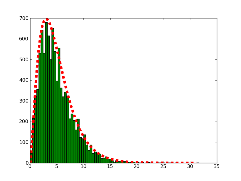
Probably the simplest example is of rolling dice. If an n-sided die is rolled many times, then the distribution of the counts for each of the n-sides should take on a chi-squared distribution (with df = n-1). I decided to simulate that in Python, with the results as shown in the graphic above. It looks pretty good to me.

Here is the code. Again, I use the Counter class from here.

import random, math from random import choice import numpy as np import matplotlib.pyplot as plt import Counter random.seed(157) class OneDie: def __init__(self,nsides=6): self.nsides = 6 self.R = range(1,nsides+1) def nrolls(self,N=100): return [choice(self.R) for i in range(N)] def chisquare_stat(N,D): stat = 0 e = 1.0 * N / len(D.keys()) for k in D: o = D[k] stat += (o-e)**2/e return stat n = 6 d = OneDie(n) L = list() N = 100 for i in range(10000): C = Counter.Counter(d.nrolls(N)) s = chisquare_stat(N,C) L.append(s) # fractional bins for the histogram width = 0.4 L = [np.floor(s/width) * width for s in L] C = Counter.Counter(L) ax = plt.axes() maxCount = C.most_common(1)[0][1] maxValue = np.max(C.keys()) ax.set_xlim(-1,maxValue+1) ax.set_ylim(0,maxCount+5) # go ahead and plot for value in C: x = value r = plt.Rectangle((x,0),width=width, height=C[value], facecolor='green') ax.add_patch(r) # chi-square should approximate gamma @np.vectorize def gamma_pdf(x,k=5): return x**(k/2.0-1) * math.e**(-x/2.0) X = np.arange(0,maxValue,0.01) Y = gamma_pdf(X,n-1) plt.plot(X,600*Y,'--', color='r',lw=6) plt.savefig('example.png')

Red card

Another set of videos from the Machine Learning Summer School 2009 features David MacKay on Information Theory (link). He poses a problem in probability which I believe is famous, but I can't find the reference now...

[UPDATE: The Box Paradox (Grinstead & Snell, p. 181)]

In his formulation, you are shown three cards. One is red on both sides, while the second is white on both sides, and a third one is red on one side and white on the other. I pick a card at random (out of sight) and show you the "up" side, which is red. What is the probability that the other side is also red?

In the class, about 50 said 1/2 and about 70 picked 2/3.

One way to solve the problem is to consider the "sample space" carefully.

Another is to write a simulation of the cards in Python. This seems to fit quite naturally with a "Card" class. We simulate a small number of draws (10⁵), and get the answer trivially (result below).

However, MacKay suggests that we solve the problem by the application of Bayes Theorem. That took me a bit to puzzle through, but after a while I came up with the following. First of all, remember Bayes' rule. We compute:

P(H|D) = P(D|H) P(H) divided by Σ P(D|H*) P(H*) for all hypotheses

What is our hypothesis? Let's say it is the event that we drew the card with two red sides, so that the side that is yet unseen is also red. What is the prior for this hypothesis? It seems uncontroversial to use the fraction of the cards which fit this hypothesis:

P(H) = 1/3

The data (or datum) is clear: one card with a red side up. What is the probability of the data we observed, given this hypothesis? Since the card is red on both sides, we have:

P(D|H) = 1

What is the marginal probability of the data, the probability under all hypotheses? This normalizing constant is:

Σ P(D|H*) P(H*) =
1/3 * 0 + 1/3 * 1/2 + 1/3 * 1 = 1/2

[UPDATE: Realized that I used the symbol * in the last line for multiplication, in the usual Python way. But H* in the line above uses * as a wildcard, to mean all H. ]

P(H|D) = P(D|H) P(H) / sum
= 1 * 1/3 divided by 1/2
= 2/3

The simulation prints:

$ python Card.py {'r': 33465, 'w': 16681}

Here's the code:

import random class Card: def __init__(self,*args): self.colors = args def __repr__(self): return ''.join(self.colors) def sideup(self): self.up = random.choice(self.colors) return self.up def sidedown(self): i = self.colors.index(self.up) if i: return self.colors[0] return self.colors[1] L = [Card('r','r'),Card('r','w'),Card('w','w')] countDict = { 'r':0, 'w':0 } for i in range(int(1E5)): c = random.choice(L) if c.sideup() == 'r': reverse = c.sidedown() countDict[reverse] += 1 print countDict