Connecting ln(x) and 1/x

I have more from Strang. We're going to look at the the limit of Δy/Δx in the context of the exponential. Following the book, we use the symbol h for Δx, the small change in x. So we have:

dy/dx = lim(h->0) [y(x+h) - y(x)] / h]

In this case, y(x) = b^x so we want

dy/dx = lim(h->0) [ bx+h - bx ] / h ]

As he says, the key idea is that we can split the first part

bx+h = bx bh

and then factor out b^x and move it outside the limit:

dy/dx = bx lim(h->0) [bh - 1] / h ]

The term in the limit is something. It depends on what the limit converges too. However, the important thing is that it is not a variable but a constant. Thus,

dy/dx = c bx

This is the equation that I used in the last post. Starting from here there is a quick demonstration of something that we proved in a more roundabout fashion before. Start with the equation above and invert it:

dx/dy = 1 / c bx

but

y = bx x = logb y dx/dy = 1/cy d/dy logb(y) = 1/cy

Beautiful! Strang says "that proof was...powerful too quick." So he does the following.

y = bx f(y) = x f(bx) = x f'(bx) (c bx) = 1 # this is the chain rule f'(bx) = 1 / (c bx) # identify bx as y f'(y) = 1/cy

f(y) converts y to x, it takes the logarithm to base b of x.

More about e

Previously I posted about a few of the remarkable properties of e, the base of natural logarithms. I said that e^x is the function that is the derivative of itself.

Actually, that's not the whole truth. Every function b^x is the derivative of itself, you just have to multiply by a constant. The thing is that the constant is 1 when b = e. As you can see in the code below, we obtain the slope of the curve b^x at x as log_e b * b^x. The constant to multiply by is log_e b, which equals 1 when b = e.

For more details, see Chapter 6 in Strang.

color.list=c( 'red','magenta', 'cyan','thistle4', 'salmon') plot(1:15,xlim=c(0.5,1.8), ylim=c(0,15),type='n') L = 2:6 L2 = c(1,1.5) for (i in 1:length(L)) { b = L[i] col=color.list[i] curve(b**x,lwd=10, add=T,col=col) for (j in 1:length(L2)) { x = L2[j] dx = 0.35 x0 = x - dx x1 = x + dx y = b**x points(x,y,pch=16, col='blue',cex=2) m = log(b)*y # slope is const * y y0 = y - m*dx y1 = y + m*dx lines(c(x0,x1), c(y0,y1),lwd=3, col='blue') } }

Slope of the sine curve

In another post about representing the sine and cosine as infinite series, I tried to show how the series form easily demonstrates the correctness of the derivatives of these functions, that if

y = sin(x) dy/dx = cos(x) y = cos(x) dy/dx = -sin(x)

But unfortunately this argument is circular (I think), since the series comes from a Taylor series, which is generated using the first derivative (and the second, third and more derivatives as well).

In this post, I want to do two things. Strang has a nice picture which makes clear the relationship between position on the unit circle and speed. This is it:



The triangles for velocity and position are similar, just rotated by π / 2.

It is clear from the diagram that at any point, the y-component of the velocity is cos(t), while the y-position is sin(t). Thus, the rate of change of sin(t) is cos(t). This is the result we've been seeking. Similarly, the rate of change of the x-position, cos(t), is -sin(t).

Strang also derives this result more rigorously starting on p. 64. That derivation is a bit complicated, although not too bad, and I won't follow the whole thing here. It uses his standard approach as follows:

dy / dx = lim(h -> 0) [sin(x + h) - sin(x)] / h

Applying a result found using just the Pythagorean theorem earlier (p. 31) for sin (s + t):

sin(s + t) = sin(s) cos(t) + cos(s) sin(t) cos(s + t) = cos(s) cos(t) - sin(s) sin(t)

He comes up with this expression for:

Δy / Δx = sin x [cos(h) - 1 / h] + cos x (sin h / h)

The problem is then to determine what happens to these two expressions in the limit as h -> 0. The first one is more interesting. As h gets small, | cos(h)-1 | gets smaller like h², so the ratio goes to 0.

R can help us see better.

h = 1 for (i in 1:6) { h = h/10 print (h) print (cos(h)-1) }

[1] 0.1 [1] -0.004995835 [1] 0.01 [1] -4.999958e-05 [1] 0.001 [1] -5e-07 [1] 1e-04 [1] -5e-09 [1] 1e-05 [1] -5e-11 [1] 1e-06 [1] -5.000445e-13

Here is the plot for the second one, which converges to 1, leaving us with simply cos(x):

f<-function(x) { x } curve(sin(x),from=0,to=0.5, ylim=c(0,0.6), lwd=3,col='red') curve(f,from=0,to=0.5, lwd=3,col='blue',add=T)

Feynman and Kepler

When I was in college I bought a book containing lectures that Richard Feynman gave at Cornell in 1964 (the Messenger series). The book is called The Character of Physical Law. Quite simply, it was and is wonderful.

Now, years later it turns out that the lectures were taped, and that after some wrangling, a famous guy (let's call him Bill) bought the rights to this material. Recently, Bill made the video available online. There's just one small problem. I promised myself I would never again install any software made by Bill and his friends on my computer. But, in order to view the lectures, he requires me to install the Silverlight plug-in for my browser (it's undoubtedly a DRM thing). In typical Bill fashion, if you go to the link for the videos, the download of the plug-in starts automatically. Long story short---I held my nose and did it. So, thanks for the lectures (link).

In Feynman's second lecture (the Relation of Mathematics and Physics) he talks about Kepler's Second Law: "A line joining a planet and the sun sweeps out equal areas during equal intervals of time." Feynman uses an argument based on vectors to show this. I didn't understand what Feynman said (and the book is just a transcription of the talk), but I googled around and found a post here. Unfortunately, the post is truncated at the critical point. The author was kind enough to write me with a detailed explanation. In the spirit of this blog as the place I post my homework for a self-taught course in anything I'm interested in, here is my version of his explanation of Feynman's explanation of Kepler's law.



Feynman uses the cross-product of two vectors.

In the diagram, the vectors A and B originate at the same point and the angle between them is θ. The cross-product A x B is a vector with magnitude = |A| |B| sin θ and its direction is perpendicular to A in the plane formed by A and B. The area of the triangle formed by A and B is one-half the magnitude of the cross-product. (I wish I knew how to produce the arrows over the labels for the vectors using html but I don't, sorry).

In the context of our problem, A is the vector from the sun to our planet at time-zero, and B is the vector at time dt. The magnitude of B is not equal to that of A, in general, because the orbit is an ellipse. So we can replace the labels by A = r and B = r + dr. The area being swept out (or its tiny component dA in a very short time dt) is proportional to the cross-product (neglect the factor of one-half):

dA = r x (r + dr)

or, as Feynman wrote using the dot notation:

. . A = r x r

Now, what we are interested in is the proposition that the rate-of-change of the area is constant, that the rate-of-change of the rate-of-change of the area is zero.

.. A = d2A/dt2 = 0

So, we need to differentiate again with respect to time, and, apparently, we can use the product rule from ordinary differentiation on this cross-product:

.. . A = d/dt (r x r) .. . . = r x r + r x r

(As Feynman says: it's just playing with dots). The second term has the cross-product of a vector with itself, θ is zero and sin θ is zero so the whole thing equals zero.

The first term has the cross-product of r with the acceleration, the rate-of-change of the rate-of-change of r with time. That is equal to F/m.

But the thing is that the force acts along the radius, so now we have the cross-product of a vector with another vector that is turned by 180° from it. This product is also zero, and therefore Ä = 0.

Area of a circle: simple calculus

I posted some time ago about a formula to find the area of the circle (knowing its circumference). I think it's credited to Euclid, although Google isn't being my friend at the moment, so I'm not sure.

To brush up on calculus, let's explore methods to find the area (as described in Strang's Calculus. He says:

"The goal here is to take a first step away from rectangles...that is our first step toward freedom, away from rectangles to rings."

In the example on the left panel of the figure, imagine slicing up the circle in the way of any standard integration problem to find the area under a curve. Simplify by considering only the area above the dotted line (y = 0). If the radius is R, then we can write y as a function of x:

y = (R2 + x2)1/2

Immediately, we run into a problem. I don't know a function which gives this as its derivative, so I don't know how to integrate it. Let's leave it until the end.

In the second approach, we picture the circle as being built up out of rings. As the radius r varies from 0 to R, the circumference of the ring is 2πr and we need to integrate:

A = ∫ 2πr dr = πr2 + C

evaluated between r = 0 and r = R:

A = πR2

As Strang emphasizes, now we can see the geometrical reason why the the derivative of the area is the circumference! How fast does the area grow? It grows in proportion to the circumference.



Exactly the same argument explains why the surface area of a sphere (4πr²) is the derivative of the volume (4/3πr³).

The third approach is to visualize the circle being sliced like a pie. This is really the same method we used in the previous post, which employed calculus on the sly. Now we have a series of triangles. The angle at the vertex of each thin triangle is dθ. The height is just R, and the base of each triangle is proportional to R, it is R dθ. So the area of the thin triangle is:

dA = 1/2 R2 dθ

We integrate (R is a constant) and evaluate between θ = 2π and θ = 0:

A = 1/2 R2 θ A = 1/2 R2 2π A = π R2

Back to the first method. We will try numerical integration. We will compute the area of the quarter-circle between x = 0 and x = R, and then simplify even further by considering just the unit circle with R = 1. We do this in a naive way, dividing the figure into a large number of thin segments, and calculate:

y = (1 - x2)1/2

We get a better approximation if we divide the very first interval in half. In R:

y <- function(x) { sqrt(1 - x**2) } d = 0.00001 x = seq(0,1,by=d) f = y(x) S = sum(f[-1]) + 0.5*f[1] S = S*d

> S [1] 0.7853982 > S*4 [1] 3.141593

Series for sine and cosine

You probably know that the sine and cosine functions can also be given as a series:

sin(x) = x - x3/3! + x5/5! - x7/7! ... cos(x) = 1 - x2/2! + x4/4! - x6/6! ...

And furthermore, that the exponential function can also be given as a series:

ex = 1 + x/1! + x2/2! + x3/3! + x4/4! ...

These series are really interesting. One reason is that they make clear that the formulas for the derivatives of these functions are obviously correct.

Take e first:

ex = 1 + x/1! + x2/2! + x3/3! + x4/4! ... d/dx ex = 0 + 1/1 + 2x/2 + 3x2/(3*2!) + 4x3/(4*3!) ... = 1 + x/1! + x2/2! + x3/3! ... = ex

Now, the sine:

sin(x) = x - x3/3! + x5/5! - x7/7! ... d/dx sin(x) = 1 - 3x2/3*2! + 5x4/5*4! - 7x6/7*6! ... = 1 - x2/2! + x4/4! - x6/6! ... = cos(x)

That's really spectacular. So the question I had was: where do these series come from. And I'm not sure this is the only way, but I think they come from a Taylor series. The Taylor series approximates a function f(x) at a particular point x = a by the series:

f(x) ≈ Σ (n=0 to n=∞) f(n)(a)/n! * (x-a)n

where f⁽ⁿ⁾(a) is the nth derivative of f(x). For e^x, all of these derivative terms are just e^x. Evaluating the series for a = 0 these derivatives are 1, and the series becomes (as we had above):

f(x) ≈ Σ (n=0 to n=∞) xn / n!

Now, I still have a couple of problems. For example, in order to get the terms of the Taylor series for sine and cosine we will have to know the derivatives, which is also what we seek, so that is a circular argument. Also, I'm not very clear on what the a is about. The approximation to f(x) works for the "neighborhood of a."

R code:

plot(1:2*pi,ylim=c(-1.2,1.2),type='n') curve(sin,from=0, to=2*pi, col='blue',lwd=5) curve(cos,from=0, to=2*pi, col='red',lwd=5,add=T) lines(c(0,2*pi),c(0,0),lty=2,lwd=3)

Duly Quoted

Here's a funny (and telling) story about a job interview someone had with Johnny von Neumann (and my post here):

"Von Neumann lived in this elegant lodge house on Westcott Road in Princeton... As I parked my car and walked in, there was this very large Great Dane dog bouncing around on the front lawn. I knocked on the door and von Neumann, who was a small, quiet, modest kind of a man, came to the door and bowed to me and said, 'Bigelow, won't you come in,' and so forth, and this dog brushed between our legs and went into the living room. He proceeded to lie down on the rug in front of everybody, and we had the entire interview---whether I would come, what I knew, what the job was going to be like---and this lasted maybe forty minutes, with the dog wandering all around the house. Towards the end of it, von Neumann asked me if I always traveled with the dog. But of course it wasn't my dog, and it wasn't his either, but von Neumann---being a diplomatic, middle-European type person---he kindly avoided mentioning it until the end."

--Julian Bigelow
quoted in:
Who got Einstein's Office
Ed Regis
p 110

Towers of Hanoi

This famous mathematical game is described in wikipedia. Briefly, we have three pegs and N disks. We wish to move the whole stack of disks to a different peg, let's say # 3. The rules are:

• Only one disk may be moved at a time.
• Each move consists of taking the upper disk from one of the rods and sliding it onto another rod, on top of the other disks that may already be present on that rod.
• No disk may be placed on top of a smaller disk.

For example, here is an intermediate stage in the game with 4 disks. Can you see the three moves that brought us to this point?



A couple of interesting things: one is the recursive nature of Towers of Hanoi. If you already know how to solve the game with N disks, then how do you solve the game with N+1?

Easy, move the first N disks to peg # 2, then move disk N+1 to peg # 3, then move all the other N disks on top. This stereotyped pattern leads to the following visual aid. (I've forgotten where I saw it). It looks like a binary ruler.



This version of the ruler describes the series of moves (though not the target pegs) for the N=4 game. To extend it, add a new bar of the correct height for N = 5, then duplicate all the bars we already have.

The number of moves grows rapidly:

N moves 1 1 2 3 3 7 4 15 N 2N-1

According to wikipedia:

The puzzle was invented by the French mathematician Édouard Lucas in 1883. There is a legend about a Vietnamese temple which contains a large room with three time-worn posts in it surrounded by 64 golden disks. The monks of Hanoi, acting out the command of an ancient prophecy, have been moving these disks, in accordance with the rules of the puzzle, since that time. The puzzle is therefore also known as the Tower of Brahma puzzle. According to the legend, when the last move of the puzzle is completed, the world will end.

We can calculate, at one move per second, this game will take roughly 292 billion years, about 20 times the current age of the universe.

>>> x = 3600*24*365 >>> x 31536000 >>> 2**63/x 292471208677L

Volume of a sphere: calculus

This derivation is straight from the book Strang's Calculus. We want to calculate the volume of a hemi-sphere as shown in the figure. The cross-sections of this solid are semi-circles. The area of each semicircle is:

A = 1/2 πr2 = 1/2 π(R2-x2)

To find the volume, we add up (integrate) the areas of each little slice:

V = ∫ A(x) dx = ∫ 1/2 π(R2-x2) dx = 1/2 π [ R2x - 1/3 x3 ]

Evaluate the expression in brackets between x = -R and +R:

= [R3 - 1/3 R3] - [-R3 + 1/3 R3] = 2/3 R3 - - 2/3 R3 = 4/3 R3 V = 1/2 π 4/3 R3 = 2/3 π R3

The total volume is twice this, or

V = 4/3 π R3

The volume can be found in either cylindrical or spherical coordinates. For spherical coordinates we have:

x = r cosθ sinφ y = r sinθ sinφ z = r cosφ

That is, φ is the angle of the vector r with the z-axis, so the z-component is r cosφ. The component orthogonal to that is the projection of r on the x,y-plane, and that is r sinφ. Then, θ is the angle of that projection (and r) with respect to the x-axis. The x- component is r sinφ cosθ (the order is not important), while the y-component is r sinφ sinθ.

In this case, the integral is a triple integral:

2π π R V = ∫ ∫ ∫ r2 sinφ dr dφ dθ 0 0 0

From reading Chapter 14 on multiple integrals in Strang, it seems that what we do here is to first integrate with respect to r, holding the angles constant:

2π π V = 1/3 R3 ∫ ∫ sinφ dφ dθ 0 0

UPDATE: A sharp-eyed reader caught a silly error in the part that follows, so it's been edited. I had set up the problem in the first half (see the figure at the beginning of the post) to use the hemisphere. But in the second part we have two angles, θ and φ, with different limits of integration.

Continuing with the standard approach in two dimensions, we let θ go from 0 to 2π. Now φ will go from 0 to π. Imagine rotating the great circle in the xy-plane around the x-axis: we need only to go from 0 to π. We could do the hemisphere by having φ go from 0 to π/2, but it would be a weird volume, with two wedges joined at the x-axis.

So, we have the integral of sinφ dφ, which is - cosφ, evaluated between φ = 0 and φ = π =>

= -cos(pi) - -(cos(0)) = -(-1) + 1 = 2 2π V = 2/3 R3 ∫ dθ 0

But this is just θ evaluated between θ = 0 and θ = 2π => 2π, so finally we have:

V = 4/3 R3 π

(Figures are from the book)

UPDATE 2: Coming back a couple of years later, I notice Google has made changes to blogger (editing the html) that retroactively messed up the formatting on this post. The limits of integration aren't shown at the correct column offset any more. My apologies, but I don't see a simple fix at the moment.

Archimedes: volume of a sphere

Archimedes was one of those rare people in the history of the world who overwhelm you with their genius. Like few others, he discovered not just one but a large number of really important things. The discovery of which he was probably most proud was the method to find the volume (and surface area) of a sphere. He found that the volume of a sphere is 2/3 the volume of the cylinder that just contains it.

This was symbolized by the sphere and cylinder on his tombstone, as witnessed (years later) by Cicero. We have no idea what Archimedes looked like, but that doesn't keep people from drawing his portrait!

What strikes me most vividly about the discovery is that Archimedes found the correct relationship by experiment---he weighed the solids, and not only that, he used the law of the lever. According to this page, the balancing was done in a fairly complex manner. We have a cylinder that can just contain the sphere and a cone whose radius and height are equal and twice the radius of the sphere. Moreover, the density of the cylinder is four times that of the other two objects.



Then, by the law of the lever, the weight of the cylinder is twice the combined weights of the sphere and the cone together (an equal force from gravity when suspended at half the distance from the fulcrum). Because the density of the cylinder is 4 times greater, its volume must be also one-half the combined volumes of the sphere and the cone.

We can check that using the (now) known formulas (see my post about the cone):

Vcylinder = 2r*πr2 = 2 πr3 Vsphere = 4/3 πr3 Vcone = 1/3 π(2r)(2r)2 = 8/3 πr3 Vsphere + Vcone = 4 πr3

According to Archimedes in the Method (translation by Heath):

"For certain things which first became clear to me by a mechanical method had afterward to be demonstrated by geometry...it is of course easier, when we have previously acquired by the method some knowledge of questions, to supply the proof than it is to find the proof without any previous knowledge. This is a reason why, in the case of the theorems the proof of which Eudoxus was the first to discover, namely, that the cone is a third part of the cylinder, and the pyramid a third part of the prism, having the same base and equal height, we should give no small share of the credit to Democritus, who was the first to assert this truth...though he did not prove it."

Once he knew the correct answer, he was able to find his way to a rigorous derivation. Very smart.

There two things that make me wonder about the story. One is: why not just weigh objects of equal density like this:



We get 4/3 for the sphere, 2/3 1/3 for the cone, and 2 for the cylinder. It should work. (Oops, see below). My guess is that Archimedes is just showing off. Note that he would have used his principle of buoyancy to determine the correct densities (and for that matter, could use the law of the lever to correct if the cylinder's density was not precisely 4x the others).

The second question is: what materials would he use? What has a density 4 times something else? From wikianswers we have:

Sand 2.80 Copper 8.63 Silver 10.40 Gold 19.30 Marble 2.56

How about marble and silver?

[UPDATE: Almost two years later, I find a silly error in this post. You'd need two cones, or put the one out at 2x the distance on the lever. Why didn't someone tell me?]

Volume of a cone: simple calculus

I've been brushing up on my calculus skills, though it can be challenging for an old fart like me. (In one ear and out the other). I saw a book online (Strang's Calculus), which I like because it is succinct, and also the author has a very interesting, idiosyncratic style. I liked it so much I got a hard copy. Now that I've studied a bit, I realize that the book is more than succinct, it's dense, filled with math, and contains a lot more than just calculus. It's a great book.

In Chapter 8, Applications of the Integral, we encounter Example 11, to find the volume of a cone. I've redrawn the diagram from the book, below. The idea is to move vertically from the top to the bottom, letting x be equal to the radius at each point. At each value for x, we draw a shell (the outside surface of a cylinder) as shown in red. As we move from top to bottom, we accumulate a collection of these cylinders whose volumes are summed to get the volume of the cone.

The key is to recognize that the distance from the top of the cone to the top of each cylinder has the same relationship to x as b does to r (e.g. when x = r, then this distance = b). The smallest and largest rectangles in the figure are similar.

The height of the cylinder plus this distance equals b.



So the height of each cylinder is

h = b-bx/r

From this point it's easy. The area of the cross-section of each shell is its diameter (2*x), times &pi times the small width dx; the volume is this area times the height. I'm going to leave out the multiplication symbol I usually use (*) for clarity:

= 2πxhdx = 2πx(b-bx/r)dx

We sum (integrate) all these cylinders:

= ∫2πx(b-bx/r) dx = ∫2πxb dx - ∫2πxb(x/r) dx = πx2b - (2/3)πx3b/r

evaluated between x = 0 and x = r:

= πr2b - (2/3)πr2b = (1/3)πr2b

Volume of a cone: geometric method

We're on the trail of Archimedes. Last time we found a formula for the sum of the squares of the integers from 1 to n:

S = n*(n+1)*(2n+1)/6

We're going to use that in a derivation of the formula for the volume of a cone. To start with, we slice the cone horizontally. In the limit as the number of slices gets very large and each individual slice gets very thin, the triangular shaped wedge pieces and the little bit at the top won't contribute significantly to the volume.

Here is the diagram from the post:

+ /|\ / |h\ +--+--+ /| |h |\ / | |r1| \ +--+--+--+--+ /| |h |\ / | | r2 | \ +--+-----+-----+--+ /| |h |\ / | | r3 | \ +--+--------+--------+--+ /| |h |\ / | | r4 | \ +--+-----------+-----------+--+ R

As Dr. Peterson explains

If the cone has base radius R and height H, and we've cut it into N slices (including that empty slice at the top, with radius r0 = 0), then each cylinder will have height h = H/N, and radius r[k] = kR/N, where k is the number of the cylinder, starting with 0 at the top and ending with N-1 for the bottom cylinder.

The only thing that's tricky about this is the numbering. The triangle at the top will be ignored. This includes the cylinder numbered k = 0 with radius = kR/N = 0. The next section below it contains a cylinder with h for its height and r1 for its radius. Since we started counting at 0, the last of the N segments has k = N-1.

The volume of each individual cylinder will be:

= π * h * rk2 = π * H/N * (kR/N)2 = π * R2 * H * k2 / N3

The total volume will be the sum of these, for all k from 0 to N-1; since only k is different from one cylinder to the next, we can factor everything else out from the sum and get:

V = [π * R2 * H / N3 ] * Sum(k2) Sum(k2) = 0 + 1 + 4 + ... + (N-1)2

Use our formula from last time:

Sum(k2) = (N-1)*(N)*(2N-1) / 6

Divide by N³:

Sum(k2) = (1-1/N)*(1)*(2-1/N) / 6

As N gets very large this converges to 2/6 = 1/3, so we have finally:

V = π*R2*H / 3

Very nice.

Sum of squares

I got interested in learning more about Archimedes. In particular, I was amazed by his derivation of the formula for the volume of a sphere. Actually he was pretty proud of it himself---according to legend and confirmed by Cicero's testimony his gravestone "was surmounted by a sphere and a cylinder."

So that's where I'm headed, but in order to get there, we need to start with a simpler problem. What is the sum of all the values n² for n = 1 to n = k? The squares and the sum go like this:

1 1 4 5 9 14 16 30 25 55 36 91 49 140 64 204

It is hard to see the pattern, so let's look up the answer, the formula is:

sum of squares = k * (k+1) * (2k+1) / 6

There is a neat proof by induction in the post. We assume that the formula is correct for n = k and then prove that if so, it is also true for n = k+1. We must also prove that it works for the "base case", n = 1, but that is self-evident.

We have:

n = k Σ n2 = k * (k+1) * (2k+1) / 6 n = 1

To find the sum of squares for k+1, we add (k+1)² to both sides. Here is the right-hand expression:

k * (k+1) * (2k+1) / 6 + (k+1)(k+1)

Factor out (k+1)

(k+1) * [ k * (2k+1) / 6 + (k+1) ] (k+1) * [ k * (2k+1) + 6k + 6 ] / 6 (k+1) * [ 2k2 + 7k + 6 ] / 6

The term in the brackets can be factored to give:

(k+2) * (2k+3)

which can be rearranged to

[(k+1) + 1] * [2*(k+1) + 1]

So we have, finally:

(k+1) * [(k+1) + 1] * [2*(k+1) + 1] / 6

which is what we wanted to prove.

There is an even better proof in the link which uses a "telescoping sum."

Duly quoted

Do you have ideas in your head that have been there forever, and then when you really need to know, where did it come from, you can't find the source? That's the way I feel about the subject of this post. I searched for the source of one such idea, but found only this:

"Life is an endless series of experiments."

---Mohandas K Gandhi (link)

While this sounds nice, of course it is fundamentally wrong. As one of my early mentors, Bart Sefton, often told me:

"Every good experiment comes with a control."

And the quote I was searching for, which I have always attributed to Milan Kundera, goes like this:

"That's the trouble with life, you never do the control."

I thought it was in The Unbearable Lightness of Being (link), but I can't find it.

The fly and the train, contd.

Thinking about the famous story involving von Neumann and the infinite series, I guessed that if we have a series where:

each succeeding term x_n+1 is produced from the preceding term x_n by multiplying by the factor 1/r, then the sum of all the terms x_n+1 + x_n+2... is equal to x_n * 1/(r-1).

So, I ran a Python simulation and it turns out to be correct!

def test(r): n = 100 # works for other n as well rL = [n] f = 1.0/r for i in range(10): rL.append(rL[-1]*f) print str(r).ljust(3), print round(n*1.0/sum(rL[1:]),2) for r in range(2,10): test(r)

2 1.0 3 2.0 4 3.0 5 4.0 6 5.0 7 6.0 8 7.0 9 8.0

If I'm reading the article correctly, this turns out to be a simple result from the theory of geometric series, and it looks like it works even for fractional r. Modifying the code above to test fractional r shows this is true. Department of "learn something new every day"....

My guess is that von Neumann saw all three pieces instantly:
• the first term and step size of the series
• the formula for the terms after the first one
• the easy way

von Neumann

I'm reading a biography of Johnny von Neumann by Norman Macrae. Or maybe I should say the biography, it's not like there are many choices for biographies of this great mathematician and early computer scientist. The book is not horrible and it's the only game in town, so I am reading it. It's based on material collected by Stephen White---who was somehow involved with Stan Ulam in an earlier version of the project.

The basic problem with the book is that Macrae is a whack job. To quote Mark Yasuda's review at Amazon:

By far the biggest problem, however, comes from MacRae's approach to the book - he insists upon inserting so much of his own world views and dogma into the body of the book, that we no longer have a biography on Von Neumann - we have Von Neumann's life used as a vehicle for MacRae's own personal views on education, politics, the Japanese economy of the 1960's through the 1980's (I never expected to see this in a Von Neumann biography), and cold war history. He takes time out to provide slanted views of Bertrand Russell and Norbert Wiener, for no reason (they barely figure in the book beyond his distorted descriptions of them) other than to insinuate that their liberal viewpoints are due to poor parenting. In sum, the book's most fatal flaw is that there's entirely too much of MacRae, and not enough Von Neumann.

Leaving all that aside, the book contains yet another retelling of the famous story about von Neumann and his approach to this problem:

Two trains (or bicycles) are 20 miles apart and headed directly toward each other at a speed of 10 mph. A fly starts from the front of the train on the left, flies at a speed of 15 mph to the tip of the train on the right, then turns around immediately and flies back to the first. This cycle continues until the trains meet, ending everything. How far does the fly fly?

The story is that when posed this problem, von Neumann thought for a second and gave the answer (below). When asked how he did it, he answered "I summed the infinite series, of course."

The easy way to do the calculation is to focus on the trains:

1. The trains will meet in one hour.
2. The fly will fly 15 miles in that hour.

What was interesting to me is that, when you think about the series method, it is not that hard, and converges rapidly.

In the first cycle the fly and its target train start with a separation of 20 miles. The fly's trajectory covers the initial distance times the ratio of its velocity to the total velocity of approach (15/(10+15)):

d1 = 20 miles * 0.6 = 12

However, each of the trains also moves 12 miles * 10/15 = 8 miles during the same period, so the new distance for the second cycle is 20 - 2*8 = 4, or one-fifth of the original. If you follow this out you can see that the series we need to sum has its first term equal to 12 and each succeeding term is 1/5 of the preceding one. The first four terms sum to:

12 + 2.4 + 0.48 + 0.096 = 14.976

I think Johnny guessed at this point.

Come to think of it, there is probably a theorem about infinite series that says if we add terms like this, the sum of all the terms obtained from 12 by multiplying by 1/5, that will be equal to 12 * 1/4. Anybody know?

[UPDATE: Not sure if this was laziness (I was in a hurry) or being incredibly dumb. See wikipedia. This is the geometric series with r = 1/5 and a = 12. The sum is a times 1/(1-r) = 12*5/4 = 15. ]

Duly Quoted

"Perhaps the worst plight of a vessel is to be caught in a gale on a lee shore. In this connection the following...rules should be observed:

1. Never allow your vessel to be found in such a predicament..."

Callingham, Seamanship: Jottings for the Young Sailor
as quoted in:
Len Deighton, Horse Under Water

Duly Quoted

From Ezra Klein:

Love is what we call it when our neuroses are compatible.

(link)

Gamma distribution

I posted previously about the beta distribution here, here and here. We ran into it because it is the conjugate prior for Bayesian analysis of problems in binomial proportion. That's because the likelihood function is in the same form.

The beta distribution is a continuous probability distribution with two shape parameters α and β (or a and b). If we consider p as the random variable (and q = 1-p), then the unnormalized distribution is just:

f(x) = pa-1 qb-1

The function has symmetry: if we switch a and b, and also p and q, everything would look the same. Varying the values for a and b can yield a wide variety of shapes. For large a and b, the plot approaches a normal distribution with mean = a / a+b.

The need to normalize the beta distribution brings us to the gamma distribution. This one can be viewed in a simple way but also can be fairly complex. The simple version is that, for positive integers, Γ(x) is just (x-1)!.

The normalizing constant for the beta distribution with parameters a and b is:

Γ(a+b) / (Γ(a) * Γ(b))

The gamma distribution is frequently used in phylogenetic models, for example, to model the distribution of variability during evolutionary time among different positions in a protein. The gamma distribution also has two parameters but these apparently have quite different roles.

They are called the shape parameter (k) and the scale parameter (θ). More generally, the unnormalized gamma distribution is:

f(x) = xk-1 exp { -x / θ }

We can get an idea of the roles of the two variables by considering this:

mean = kθ variance = kθ2

Let's look at some plots obtained using different values for the two parameters. In the series below, k goes from 1 to 4, and then for each plot theta varies from 0.25, 0.5, 1, 2, 3 as the color goes from blue to green to magenta to red to maroon.

N = 6 thetaL = c(0.25,0.5,1,2,3) color.list = c('blue','darkgreen', 'magenta','red','darkred') #k = 1,2,3,4 plot(1:N,ylim=c(0,0.8),type='n') for (i in 1:5) { curve(dgamma(x, shape=k,scale=thetaL[i]), from=0,to=N,lwd=3, col=color.list[i],add=T) }

Geometric distribution

According to wikipedia, the geometric distribution is the probability distribution which describes the number of Bernoulli trials required to obtain a single success.

So, in the simple case of a fair coin (p = 1/2):

P(X=1) = 1/2 P(X=2) = 1/4 (1/2 times 1/2) P(X=3) = 1/8 (1/2 times 1/4)

According to mathworld, the geometric distribution is the only discrete memoryless random distribution, and is a discrete analog of the exponential distribution.

The memoryless property can be seen easily if we take the geometric series:

1/2 + 1/4 + 1/8 ...

If we have already obtained a failure on the first trial, then we remove the first term (corresponding to success on the first trial) and then normalize by dividing by the sum of all remaining terms (1 - 1/2):

= 2/4 + 2/8 + 2/16 ... = 1/2 + 1/4 + 1/8 ...

The normalization is needed because we require the sum of all the terms to add up to 1 for a proper probability distribution. In general, for process with probability of success p and failure q = 1 - p:

P(X=k) = qk-1 * p

According to wikipedia, the mean is 1/p and the variance is q/p². We can compare that to the exponential distribution with a pdf of:

λe-λx

and mean = 1/λ and variance = 1/λ².

It is not clear to me at present why the expressions for the variance don't match up.

R code:

x=numeric(7) x[1] = 1 for (i in 2:length(x)) { x[i] = x[i-1]/2 } plot(x,type='s', ylim=c(0,1.0), col='red',lwd=3)

Normally squared

According to wikipedia, the chi-square distribution (with df = k), arises as the sum of the squares of k independent, normally distributed random variables with mean 0 and variance 1. For example, in a bivariate distribution where each variable is normally distributed, the square of the distance from the origin should be distributed in this way with df = 2.

u = rnorm(10000) v = rnorm(10000) w = u**2 + v**2 B = seq(0,max(w)+1,by=1) hist(w,freq=F,ylim=c(0,0.5), breaks=B,col='cyan') curve(dchisq(x,df=2), lwd=5,col='red', from=0,to=10,add=T)

I found that I could also get the chi-squared distribution by multiplying two random variables (with mean not equal to 0) together, and it seems that in this case the degrees of freedom is equal to the product of the means.

u = rnorm(10000,3) v = rnorm(10000,3) w = u*v B = seq(-5,max(w)+1,by=1) hist(w,freq=F,ylim=c(0,0.18), breaks=B,col='cyan') curve(dchisq(x,df=9), lwd=5,col='red', from=0,to=30,add=T)

Let's explore how to use R to solve the problem of the grade distribution from the last post. We have males and females with grades from A,B,D,F in order, stored in a matrix M:

m = c(56,60,43,8) f = c(37,63,47,5) M = t(rbind(m,f))

> M m f [1,] 56 37 [2,] 60 63 [3,] 43 47 [4,] 8 5

r = chisq.test(M)

> r Pearson's Chi-squared test data: M X-squared = 4.1288, df = 3, p-value = 0.2479

This matches the value given in Grinstead & Snell. We can explore contributions of the individual categories to the statistic as follows.

E = r$expected O = r$observed (O-E)**2/E

We see that the disparity in A's was certainly higher than for the other categories, but the p-value (above) is not significant.

> (O-E)**2/E m f [1,] 1.0985994 1.2070139 [2,] 0.2995463 0.3291068 [3,] 0.3595670 0.3950506 [4,] 0.2096039 0.2302885

We see that the 95th percentile of the chi-squared distribution for df=3 is just a bit larger than 7.8:

> S = seq(7,8,by=0.1) > pchisq(S,df=3) [1] 0.9281022 0.9312222 0.9342109 0.9370738 [5] 0.9398157 0.9424415 0.9449561 0.9473637 [9] 0.9496689 0.9518757 0.9539883

We can do a Monte Carlo simulation (I actually do not know yet how the preceding function works, but the simulation should be just like what we did yesterday:

r = chisq.test(M,simulate.p.value=T)

> r Pearson's Chi-squared test with simulated p-value (based on 2000 replicates) data: M X-squared = 4.1288, df = NA, p-value = 0.2414

And Fisher's exact test (also on my study list for the future):

r = fisher.test(M)

> r Fisher's Exact Test for Count Data data: M p-value = 0.2479 alternative hypothesis: two.sided

Grade disparity - chi-squared analysis

I recently posted about two common statistical problems: the first involves making an estimate of the population mean when the sample size is small, involving the t statistic of "Student", as well as the related problem of deciding whether the means for two small samples are different, including the example of paired samples. These arise commonly in biology. The second problem is deciding whether two sets of paired values are independent, or instead whether given the value for x, we can predict y. This problem involves covariance and the simplest approach is linear regression.

The third basic problem in statistics for which I want to improve my understanding is that of the independence of two discrete distributions. This will lead us to the chi-squared density as a special case of the gamma distribution.

There is a very nice discussion of this in Grinstead & Snell (pdf). Here is their table which gives a grade distribution, comparing the results for females and males in a particular class.



If the distributions are independent (e.g. P(grade = A) = P(grade = A | sex = female), then we can predict the most likely distribution, but also expect that there will be some spread in the observed breakdown by grade and sex due to random sampling. How much deviation should we expect?



We can model the problem using colored balls. For example, we put 152 pink balls and 167 baby blue balls in to an urn, mix well, and then draw out in succession 93 'A's, 123 'B's, 90 'C's and 13 'D's.

We calculate for each category:

(O - E)²/ E

where O is the observed value and E the expected value based on the assumption of independence. We sum the value over all categories to obtain the statistic. According to theory, this statistic has a chi-squared (Χ²) distribution with degrees of freedom df = 3. (For this problem df is the number of grades - 1 * the number of sexes - 1).

If the calculated value for the statistic exceeds 95 % of the values in the distribution for this df, we reject the null hypothesis that the two probability distributions are independent. In other words, we suspect that males and females have different grade distributions for this course.

For this data, the value of Χ² that is exceeded 5 % of the time is 7.8, so the calculated value of 4.13 does not allow rejection.

Here is code for a Python simulation (R code to plot is at the end). I redirect the output to a file like so:

python grades.py > results.txt

import random rL = list() # for statistic values F = 152; M = 167 N = M + F f = F*1.0/N; m = M*1.0/N v = False grades = [93,123,90,13] # expected values: EF = [f*g for g in grades] EM = [m*g for g in grades] def test(): print 'EF', for e in EF: print round(e,2), print print 'EM', for e in EM: print round(e,2), print R = 10000 # number of trials for i in range(10000): if v: test() chisq = 0 pL = ['F']*F + ['M']*M random.shuffle(pL) mL = list() fL = list() for i in range(4): # grades A-D n = grades[i] # how many 'A's... fL.append(pL[:n].count('F')) mL.append(pL[:n].count('M')) pL = pL[n:] if v: print 'OF',' '.join([str(e).rjust(2) for e in fL]) if v: print 'OM',' '.join([str(e).rjust(2) for e in mL]) for i in range(4): chisq += (fL[i]-EF[i])**2/EF[i] chisq += (mL[i]-EM[i])**2/EM[i] print round(chisq,2) if v: print

setwd('Desktop') v = read.table( 'results.txt',head=F) B = seq(0,20,by=0.25) hist(v[,1],freq=F,breaks=B) curve(dchisq(x,3), from=0,to=20,add=T,col='blue',lwd=3)

Regression corrected

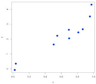
If you read my post about regression from yesterday, you may have noticed that it has a serious problem with the way the errors were generated. What I did was this:

set.seed(157) x = runif(10) e = x for (i in 1:length(x)) { e[i] = rnorm(1,mean=x[i],sd=0.3) } y = 2.4*x + e plot(y~x,pch=16,col='blue',cex=1.8)

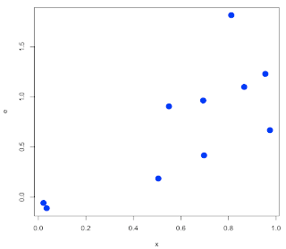
If we look at the errors, we see that they are dependent on the value of x! Naturally (b/c of mean=x[i]).

plot(x,e,pch=16,col='blue',cex=2)

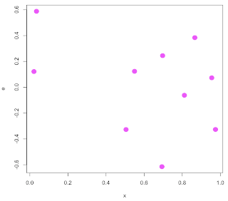
What I should have done is something like this:

set.seed(1357) e = rnorm(10)/3 y = 2.4*x + e plot(x,e,pch=16,col='magenta',cex=2)

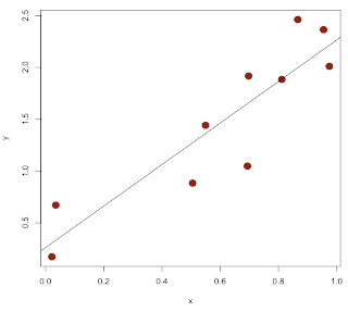
plot(x,y,pch=16,col='darkred',cex=2)

Nevertheless, I hope the essential points are clear:

• covariance is related to variance: cov(x,x) = var(x)
• correlation is the covariance of z-scores
• the slope of the regression line is: cov(x,y) / var(x)
• the regression line goes through x, y
• r ≈ cov(x,y) / sqrt(var(x)*var(y))
• the call to plot the line is abline(lm(y~x))

The proportionality for r is b/c we are not matching R's output for this. I think it is because we are missing a correction factor of n-1/n. I will have to look into that when I get back to my library at home.

With the change, we do a little better on guessing the slope:

> lm(y~x) Call: lm(formula = y ~ x) Coefficients: (Intercept) x 0.2625 2.0039

Limited power

I first came across Andrew Gelman's name because he co-wrote a book called 'Red State, Blue State'. I'm interested in politics and follow a few bloggers I think are smart---funny that they all turn out to be "progressives." What are the chances?

I haven't read that book, though I do have a book of his with ideas for teaching Statistics, and I aspire to read his book on Bayesian Analysis. He also has a blog.

Anyway, somewhere I came across an article of his on the web (pdf). It's an analysis prompted by the publication of a set of articles in the Journal of Theoretical Biology with titles such as "Beautiful Parents Have More Daughters," that are (as you might guess by this point) fatally flawed. It's a great read.

Basic regression

Continuing with my education in statistics, I'm reading Dalgaard's book, Introductory Statistics with R. The topic of this post is linear regression by least squares.

We're going to model errors in the data as follows:

set.seed(157) x = runif(10) e = x for (i in 1:length(x)) { e[i] = rnorm(1,mean=x[i],sd=0.3) } y = 2.4*x + e plot(y~x,pch=16,col='blue',cex=1.8)

[UPDATE: this is not the correct way to model the errors. See here.]

dx = x-mean(x) dy = y-mean(y) n = length(x) sum(dx**2)/(n-1) var(x)

The variance of x is computed in the usual way:

> sum(dx**2)/(n-1) [1] 0.1182592 > var(x) [1] 0.1182592

The covariance of x and y is defined in such a way that the variance of x is equal to the covariance of x with itself. That makes it easy to remember!

sum(dx*dy)/(n-1) cov(x,y)

> sum(dx*dy)/(n-1) [1] 0.4309724 > cov(x,y) [1] 0.4309724

Correlation is just like covariance, only it is computed using z-scores (normalized data).

zx = (x-mean(x))/sd(x) zy = (y-mean(y))/sd(y) cov(zx,zy) cor(x,y)

> cov(zx,zy) [1] 0.9515839 > cor(x,y) [1] 0.9515839

As discussed in Dalgard (Ch. 5), the estimated slope is:

β = cov(x,y) / var(x)

> cov(x,y) / var(x) [1] 3.644302

while the intercept is:

α = y - β*x

The linear regression line goes through x, y.

Let R do the work:

> lm(y~x) Call: lm(formula = y ~ x) Coefficients: (Intercept) x -0.04804 3.64430

The estimated slope is 3.64, while the true value is 2.4. I thought the problem was the last point, but it goes deeper than that.

># doing this by hand > i = 7 # index of max y value > lm(y[-i]~x[-i]) Call: lm(formula = y[-i] ~ x[-i]) Coefficients: (Intercept) x[-i] -0.1053 3.5803

Much more information is available using the "extractor function" summary:

> summary(xy.model) Call: lm(formula = y ~ x) Residuals: Min 1Q Median 3Q -0.456059 -0.369435 -0.006057 0.239960 Max 0.814548 Coefficients: Estimate Std. Error t value (Intercept) -0.04804 0.28819 -0.167 x 3.64430 0.41621 8.756 Pr(>|t|) (Intercept) 0.872 x 2.27e-05 *** --- Signif. codes: 0 ‘***’ 0.001 ‘**’ 0.01 ‘*’ 0.05 ‘.’ 0.1 ‘ ’ 1 Residual standard error: 0.4294 on 8 degrees of freedom Multiple R-squared: 0.9055, Adjusted R-squared: 0.8937 F-statistic: 76.67 on 1 and 8 DF, p-value: 2.267e-05

The correlation coefficient is

r = sum(dx*dy) / sqrt( sum(dx**2) * sum(dy**2) )

That is

r = cov(x,y) / sqrt(var(x)*var(y))

> cov(x,y) / sqrt(var(x)*var(y)) [1] 0.9515839

I am not sure why this doesn't match the output above.

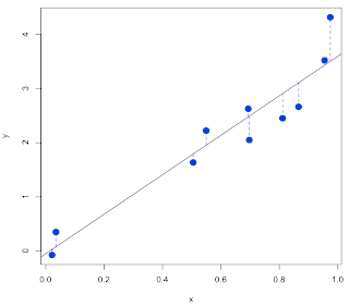
To get the plot shown at the top of the post we use another extractor function on the linear model:

xy.model = lm(y~x) w = fitted(xy.model)

w contains the predicted values of y for each x according to the model.

plot(y~x,pch=16,col='blue',cex=1.8) xy.model = lm(y~x) abline(xy.model) segments(x,w,x,y,col='blue',lty=2)

We can do an even fancier plot, with confidence bands, as follows.

df = data.frame(x) pp = predict(xy.model,int='p',newdata=df) pc = predict(xy.model,int='c',newdata=df) plot(y~x,pch=16,col='blue',cex=1.8) matlines(x,pc,lty=2,col='black') matlines(x,pp,lty=3,col='black')

This is promising but it is obviously going to take more work.