Friday, July 31, 2009

Collisions in 2D


I want to continue with the analysis of inelastic collisions between particles in two dimensions. I plan to use these for simulations. As we did previously, I will use the notations M and m to refer to two masses which will have a historic meeting. In the diagram, they approach each other in a reference frame where (i) m is at rest and (ii) all of M's velocity is along the x-axis.

To simplify things, I will only consider the case where the masses are equal, M = m. M is the blue circle in the diagram, it approaches m with velocity a. After the collision, M is deflected along angle φ below the x-axis, while m exits with angle θ above the x-axis. We use the same conservation laws which give us three equations:


(1) a = c cosφ + d cosθ
(2) c sinφ = d sinθ
(3) a2 = c2 + d2

Rearrange (1) and square it:
a2 - 2 a c cosφ + c2 cos2φ = d2 cos2θ

then add to the square of (2):
a2 - 2 a c cosφ + c2 cos2φ + c2 sin2φ = d2 cos2θ + d2 sin2θ

use the trigonometric identity
sin2α + cos2α = 1
reduce the above to:
a2 - 2 a c cosφ + c2 = d2

substitute for a2 from 3:
c2 + d2 - 2 a c cosφ + c2 = d2
rearrange:
2c2 = 2 a c cosφ

if c ≠ 0, then:
c = a cosφ

substitute for c2 in (3):
a2 = a2 cos2φ + d2
d2 = a2 (1 - cos2φ)
d2 = a2 sin2φ
d = a sin φ


So, we have solved for c and d in terms of a and the angle φ. Unfortunately, what we will know in our simulation is the positions of the two centers of mass at the moment they touch (i.e. θ). Now, we could go back and solve for θ directly. But I will assert that the following is true by symmetry:

c = a sinθ
d = a cosθ


(There is nothing special about the labels on the particles, so if we switch c and d, as well as θ and φ it should be OK).


Notice that we now have:

d = a sinφ = a cosθ
sinφ = cosθ
φ + θ = π/2


For equal masses, the particles always move away from each other at right angles.

For the x and y-components of the velocities:
cx = c cosφ = c sinθ = a sin2θ
cy = c sinφ = c cosθ = a sinθ cosθ

dx = d cosθ = a cos2θ
dy = d sinθ = a sinθ cosθ


And, as a special bonus, we notice that the 2D case also applies to 3D, because any 3D collision involves two particles whose frame of reference can always be rotated and translated so as to reduce to the 2D case. Next: using these simple equations to simulate a 2D gas.

Massive collisions

I found this simulation of a two-dimensional gas very entertaining, and also relevant in light of Maxwell's use of the rotational symmetry argument in his derivation of the Maxwell-Boltzmann distribution. I thought it would be interesting to try to program this simulation in Python. And, if it turns out that we need to speed things up, it would provide an opportunity to explore those issues as well. I know this isn't Bioinformatics, but it is all part of a plan for me to improve my math skills. In fact, I think Bioinformatics would be better called Statistical Genetics. Unfortunately, some other folks have already appropriated the term.

To begin with, I needed to dig out Halliday & Resnick, and review the equations for collisions. There is a newer edition but I used my old book, which I re-purchased some years ago from Abebooks. I want to show the derivations of the equations for collisions between two particles in one and two dimensions. Here is a graphic to motivate us:


In the one dimensional case, of course, we do not have the angles θ and &phi. We just have masses M and m, and velocities before and after collision. These are usually designated v1i, etc. but I am going to use non-standard notation to reduce my confusion, and as a bonus, simplify the typing. We will label the velocities of the masses before collision as a (for M) and b (for m), while afterward they will be c (for M) and d (for m).

We use two of the great conservation principles of physics, for momentum and energy.

In one dimension (inelastic collision), we have:
(1)  M a + m b = M c + m d
(2) 1/2 M a2 + 1/2 m b2 = 1/2 M c2 + 1/2 m d2

from (1):
M a - M c = m d - m b
(3) M (a - c) = m (d - b)

from (2)
M (a2 - c2) = m (d2 - b2)
factor:
M (a + c)(a - c) = m (d + b)(d - b)

and divide by (3), assuming a ≠ c and b ≠ d:
a + c = d + b

rearrange:
(4) a - b = d - c


Halliday & Resnick:
This tells us that in an elastic one-dimensional collision, the relative velocity of approach before collision is equal to the relative velocity of separation after collision.


(3) M (a - c) = m (d - b)

Rearrange (4) to solve for d and substitute into 3:
M (a - c) = m (a - b + c - b)
M a - M c = m a - 2 m b + m c

Rearrange terms to group by velocity:
(M - m) a + 2 m b = (M + m) c

M - m 2m
c = ----- a + ----- b
M + m M + m


We could also solve for d, but I will just assert that the following is true by symmetry:

    m - M      2M
d = ----- b + ----- a
M + m M + m


(There is nothing special about m and M, so if we switch them as well as a and b, it should be OK).

Special cases of interest.

If the masses are equal, M = m and:

d = a and c = b

The particles simply exchange velocities.

Another case is where M (say) is initially at rest, then a = 0 and


2m m - M
c = ----- b d = ----- b
M + m M + m


Now, for equal masses, then d = 0 and M simply acquires the velocity of m, while m stops abruptly.

However, if M is at rest and the masses are greatly unequal, (M >> m), then the velocity of M after the collision is still c ≈ 0, and d = -b, the small particle reverses its velocity. It just bounces off.

I'll do the 2D case in another post, and then move on to the simulation.

Wednesday, July 29, 2009

Approaching Normal

This post continues with the theme of exploring the normal distribution. I wanted to take a look at how fast repeated samples from a uniform distribution approach the normal, and in the process exercise my R skills a bit. If you have not used R, I recommend it for graphics and exploring statistics. It works well (and looks beautiful) on my Mac. In the course I taught in Spring, there was a student who had trouble installing it under Windows, but that machine was hosed anyway. Disclaimer: I am not an R guru. If I'm not "doing it right", let me know.

The first thing is to model rolling a standard six-sided die. We want to sample from the uniform distribution of integers between 1 and 6. Don't forget to sample with replacement. As usual, I use yellow background for my code, and blue background to show what the program prints to the screen.

d = 1:6
u = sample(d,10000,replace=T)
mean(u)
var(u)


As we expect, the mean or expected value is 1/6 * (1 + 2 + 3 + 4 + 5 + 6) = 21/6 = 3.5 and the variance is 1/6 * 2 * (0.52 + 1.52 + 2.52) = 1/3 * (0.25 + 2.25 + 6.25) = 1/3 * 8.75 = 2.92, and the (population) standard deviation is √2.92 = 1.71.

> mean(u)
[1] 3.4786
> var(u)
[1] 2.917434
> sd(u)
[1] 1.708050
> summary(u)
Min. 1st Qu. Median Mean 3rd Qu. Max.
1.000 2.000 3.000 3.479 5.000 6.000


We will take a look at the distribution of the numbers using the hist function. There are a couple of details to consider when using hist. (I often have to remind myself about its arguments by doing "?hist"). One is the argument "breaks"

breaks  one of:
a vector giving the breakpoints between histogram cells,
a single number giving the number of cells for the histogram,
a character string naming an algorithm to compute the
number of cells (see ‘Details’),
a function to compute the number of cells.
In the last three cases the number is a suggestion only.


I often specify the number of cells explicitly, especially when I want to compare multiple plots. Since I had a little trouble with this plot, I tried a couple of different things, and I want to plot them all in the same window. For this, I use the formatting command "par" and tell it to make a set of plots in 1 row and 3 columns.

par(mfrow=c(1,3))
hist(u,breaks=6,col='blue')
hist(u,right=F,
breaks=6,col='blue')
hist(u-0.5,breaks=6,col='blue')


As you can see, the first two histograms look funny. What is going on is that R is trying to bin the numbers in the vector with breakpoints exactly on the integer values 1, 2, 3... Since the numbers are themselves drawn from 1, 2, 3... it has to go right or left, and at the boundaries of the plot it looks weird. One argument controlling how this works is:

right  logical; if TRUE, the histograms cells are right-closed
(left open) intervals.


The default setting is "TRUE", which has cells formed as "right-closed (left-open) intervals"---whatever that means. The result is that at the left boundary all the values "1" and "2" have been binned together. Neither setting for "right" is what we want. My solution was to shift all the values to the left by 0.5 and then plot the result. The "1"s are plotted in the cell between 0 and 1.

Now, let's see what happens if we roll the dice again. What we're going to do is start with a vector of the size we need called z, that is filled with zeroes. (It has a length of 50,000). We need to initialize it because we will be updating at each round. We roll the dice six times and plot the results at each stage.


As you can see, we already have a reasonable approximation to the normal after summing just two numbers drawn at random from the "sample space" of 1, 2... , 6. And by n=6 the approximation is very good. Since the standard deviation goes as √variance, and the variances add, by n=6 we have a range of 31 (from 6 to 36) but the sd is only √(6*2.91) = 4.18 (4.19 in the figure).

Here is the code:

d = 1:6
par(mfrow=c(3,2))
z = rep(0,50000)
for (i in 1:6) {
B = i*6
z = z + sample(d,50000,replace=T)
w = z+0.5
hist(w,breaks=B,
xlim=c(min(w)-2,max(w)+2),
col='gray90',freq=F,
main=paste('sd = ',
round(sd(w),2),sep=""),
xlab=paste('round',i))
plot(function(x) dnorm(x,mean(w),sd(w)),
0,max(w),lwd=2,add=T,col='red')
}


I found the code for the function that plots the normal distribution with the same mean and sd as our samples somewhere on the web. It is doing something a bit funny. I think it is making an "anonymous" (i.e. unnamed) function to feed to plot, and then applying that function with bounds = 0 and max(w), but I'm not real clear about how this works. The parameter lwd is for line width.

Finally, let's look a little more closely at the z vector after 6 rounds. We plot it in the same histogram as the normal density of the same mean and sd, switching which one is in back as we move from the left panel to the right.


The code:

mean(z)
sd(z)
summary(z)
x=rnorm(length(z),mean(z),sd(z))
summary(x)

par(mfrow=c(1,2))
hist(z,breaks=40,freq=F,
xlim=c(0,40))
hist(x,col='gray80',breaks=40,
freq=F,add=T)

hist(x,col='gray80',breaks=40,
freq=F,xlim=c(0,40))
hist(z,col='white',
breaks=40,freq=F,add=T)


Notice, however, that the correspondence is not perfect, as shown by the results of calling the summary function.

> mean(z)
[1] 21.00562
> sd(z)
[1] 4.155018
> summary(z)
Min. 1st Qu. Median Mean 3rd Qu. Max.
7.00 18.00 21.00 21.01 24.00 36.00
> x=rnorm(length(z),mean(z),sd(z))
> summary(x)
Min. 1st Qu. Median Mean 3rd Qu. Max.
3.297 18.210 20.980 20.990 23.780 38.350


Our vector z seems a little fatter at the first and third quartiles and yet its minimum and maximum values are closer to the mean than the true normal distribution.

Tuesday, July 28, 2009

Normal approximation to the binomial


I know that the normal can be used as an approximation to the binomial. I was looking for a derivation of this, and I found it via google in a math forum. Doctor Anthony begins:


Derivation of the Normal distribution from the Binomial distribution
---------------------------------------------------------------------

Let a variate take values 0, k, 2k, 3k, ..., nk
with probabilities given by successive terms of
(q + p)^n.


What's with the k? Well, we're eventually going to want non-integer terms. The expansion of (q + p)n is familiar:

qn + nqn-1 p + n(n-1)/2 qn-2 p2 + ...


The ith term of the expansion is C(n,i).

Then the mean m = npk and the variance s^2 = npqk^2


OK. Notice use of the multiplication rule for variance from the other day.


Suppose:

y = probability of occurrence of rk = C(n,r) p^r q^(n-r)

Also let:

y' = probability of occurrence (r+1)k = C(n,r+1)p^(r+1) q^(n-r-1)

Then:

y' - y = C(n,r+1)p^(r+1) q^(n-r-1) - C(n,r)p^r q^(n-r)

n!p^r q^(n-r-1)
= ---------------[(n-r)p - (r+1)q]
(r+1)! (n-r)!


Hmm... I know that

  y =   [n! /  r!    (n-r)!]     pr     qn-r
y' = [n! / (r+1)! (n-r-1)!] pr+1 qn-r-1
y' - y = ?


Lucie, you got some factoring to do. Let's deal with q and p first.

The left term has qn-r-1 and the right term has qn-r, so we can factor out
qn-r-1, leaving a factor of q on the right-hand term in the brackets.

Similarly we can factor out pr from both sides leaving a factor of p on the left.

The combination expressions expand as shown above. We can factor out n! from both sides. We can factor out 1/(r+1)! from both sides, if we first multiply top and bottom of the right-hand term by (r+1), leaving (r+1) on the top.

Similarly, we can factor out (n-r)! from both sides, if we first multiply top and bottom of the left-hand term by (n-r), leaving (n-r) behind on the top. So everything checks out so far. Next, he wants to divide by y:


And:

y' - y 1 1
------ = ------[np - r(p+q) - q] = ------[np - r - q]
y (r+1)q (r+1)q

(Equation 1)


Hmm...again. We're dividing the expression we had above by y.

  y =   [n! /  r! (n-r)!]        pr     qn-r


We have:

             n!pr qn-r-1
y' - y = ---------------[(n-r)p - (r+1)q]
(r+1)! (n-r)!


So both n! and (n-r)! terms cancel. We also cancel r!, leaving a factor of (r+1) on the bottom. The pr cancels, and the qn-r also cancels leaves a factor of q on the bottom. So I get:

   y' - y      1
------ = ------[(n-r)p - (r+1)q]
y (r+1)q


Now we have to figure out how to rearrange the term in brackets:

  [(n-r)p - (r+1)q]


Expand, and then substitute for p + q = 1:

  np - rp - rq - q
np - r(p+q) - q
np - r - q


It checks out. Doctor Anthony continues:


Let:

x = rk - npk, so that x is now the variate measured
from the mean.

Then:

r = x/k + np and r+1 = x/k + np + 1

Thus:

k(r+1) = x + k + npk

k^2 (r+1)q = (x + k + npk)qk


So far so good.


Multiply top and bottom of the righthand side of Equation 1 by k^2. 
Then:

y' - y [(np-r)k - qk]k
------ = --------------- [note that (np-r)k = -x]
y [x + k + npk]qk


Go back to what we had, and then multiply top and bottom by k2:

   y' - y    [np - r - q] k^2
------ = ----------------
y (r+1)q k^2


Hmm... The top is fine, but on the bottom we had

(r+1) q k2


We need to get to:

[x + k + npk]qk


He says:

[note that (np-r)k = -x]


OK, so we have:

(r+1) q k2
(rk + k) q k

Since:
(np - r) k = -x
rk = npk + x

Substituting:
(x + k + npk) q k


Moving on to substitute for (np-r) k = -x on top and multiplying out on the bottom yields:

              (-x - kq)k
= ----------------
npqk2 + (x+k)qk


Finally, we now let k = dx, so that y' - y = dy and 
let n ->infinity in such a way that nk^2 is finite.
Equation 2 can then be written as:

dy (-x - q dx)dx
---- = ----------------
y s^2 + (x+dx)q dx


The only tricky part here was that we've replaced npqk2 by s2.
Now he says:

As dx -> 0 this becomes:

dy -x dx
---- = ------
y s^2


And we're there! If we integrate the left side we get ln(y), and the right side is
-x2 / 2s2

y = A exp { -x2 / 2s2 }

Gaussian normalizing constant

Last time we followed a derivation for the normal or Gaussian distribution that gave us the general form:

p(x) = A exp { -x2/2V }


What we need to do now is to evaluate the constant A. As I'm sure you remember, it has something to do with π, more accurately with √(2π). The constant doesn't really change the distribution (e.g. the fraction of the density that lies between x = +σ and x = +∞). What the constant does is to "normalize" the values so that the total density over the range of x (from -∞ to +∞) to equals one, a requirement for a real probability density function. It squishes the graph in the y-dimension. It is probably obvious that, if the total value (∫ exp { -x2/2V } over the whole range = 1/A, then multiplying by A will normalize it.

The V in the formula above turns out to be the variance of the distribution. It's usually written as σ2 but I want to leave it as it is. Let us start with V = 1 and then explore the influence of V separately. That means σ also equals one.

We can evaluate the constant A easily using R. Since the function is symmetrical, we can integrate between 0 and +∞, and then multiply the result by two. We're going to do two things to simplify our lives. First, rather than integrate, we will sum a bunch of small intervals. Second, rather than go to +∞, we will only go as far as there is significant density. Remembering the rules for z-scores, you can guess that we'll get 99% accuracy if we go out to 3*σ. Let's aim even higher and go to 5*σ.

T = 5
I = 0.1
x = seq(0,T,by=I)
x = x + I/2
x = x[-length(x)]
head(x)


> head(x)
[1] 0.05 0.15 0.25 0.35 0.45 0.55


We specify the intervals using the variable I. Here I = 0.1, but you can make it smaller if you wish. We construct a vector v which has the values between 0 and T with a spacing of I = 0.1. The sums are more accurate if we bump out all the values in the vector by I/2 (and then remove the last one, which is outside the interval we want to measure. A single interval looks something like this.


We approximate the area of the triangle on the left (red side) by the area of the triangle on the right. We calculate the vector of areas of all the slices and store the result in y, then sum over y. We multiply by 2 to adjust for the symmetrical values for -x.

y = I * exp(-0.5*x**2)
k = 2*sum(y)
k
sqrt(2*pi)


Because we know the true value, we can compare our answer it.

> k
[1] 2.506627
> sqrt(2*pi)
[1] 2.506628


We can also generalize the above code by explicitly including V. Trying different values of V, it is clear that the constant k is actually √(2 π V), and the A in the density function is 1/k. Note the use of √V = σ in the definition of T.

V = 16
T = 5*sqrt(V)
I = 0.1
x = seq(0,T,by=I)
x = x + I/2
x = x[-length(x)]
y = I * exp(-0.5*x**2/V)
k = 2*sum(y)

sqrt(2*pi)
sqrt(2*pi*V)


> k
[1] 10.02651
> sqrt(2*pi)
[1] 2.506628
> sqrt(2*pi*V)
[1] 10.02651


Dan Teague's derivation (pdf) evaluates A using calculus. I just wanted to indicate the way π creeps in. Here are some equations from him:


The double integral over x and y (equation 3) is converted to an integral in radial coordinates. The ∫ θ then contributes the π And since the conversion to radial coordinates involved x times y, going back to p(x) gives us √π. I don't know enough to be sure this is OK, but it certainly looks reasonable.

Monday, July 27, 2009

The normal (Gaussian) distribution

I'm not very good at proofs, but I wanted to try to understand where the normal distribution comes from. In fact, we saw in an earlier post that we can show by simulation that the Central Limit Theorem seems to be correct. Regardless of the underlying distribution, the sample mean x is normally distributed if the sample size is sufficiently large.

However, let's try this argument, which is originally due to Sir John F. W. Herschel.

Imagine that you are throwing darts at the origin of the x,y plane. Under perfect conditions, you would hit the center dead on every time. However, conditions aren't perfect. The wind is gusting, the music is loud, your blood alchohol is modestly elevated, there are other distractions. As a result, small errors creep in and the pattern over time looks like so:


The R code:

x=rnorm(1000)
y=rnorm(1000)
L=c(-3,3)
plot(x,y,pch=16,xlim=L,ylim=L,col='blue')
lines(c(0,0),c(-3,3),lty=2,lwd=2)
lines(c(-3,3),c(0,0),lty=2,lwd=2)


Now, there is some unknown function for the probability that a dart will land in the interval between x and x + ∆x. Obviously, the probability depends on x, with a maximum at x = 0 and then decreasing to zero as x gets large. We designate that function as a probability density function p(x) and evaluate the density over the interval to get the probability that the dart lands in the interval:


Prob = p(x) ∆x


Now we consider a small area of size ∆x∆y. If:

the errors in perpendicular directions are independent
then we expect that p(x) = p(y) and we can get the probability that a dart lands in the small rectangle bounded by x, y and x + ∆x, y + ∆y as:

Prob = p(x)∆x p(y)∆y


In fact, if we assume that the errors do not depend on the orientation of the coordinate system, then the probability is a function only of r, the radial distance from the origin, so we can write

Prob = g(r)∆x∆y
g(r)∆x∆y = p(x)∆x p(y)∆y
g(r) = p(x) p(y)


This assumption of rotational independence will lead us directly to the answer, as you will see. As Hamming says, since r does not depend on the angle θ, (but x and y do), we can take the partial derivative with respect to θ of g(r) and set it equal to zero, so that:


We can parse this. We used the standard multiplication rule (twice): "this times the derivative of that plus that times the derivative of this." We use it to generate the first line (taking the partial derivative of p(x) p(y)). And then, we need to actually find the partial derivatives of p(x) and p(y) with respect to θ, where x = r cos(θ) and y = r sin(θ). We use the multiplication rule again, and the fact that the derivative of the sine is just the cosine, while the derivative of the cosine is minus the sine. Thus, for example, the partial derivative of x with respect to θ is simply -y.

As stated, this gives:

p(x) p'(y)(x) - p(y)p'(x)(y) = 0
p'(x)/x p(x) = p'(y)/y p(y)


Since x and y are both variables:

p'(x)/x p(x) = p'(y)/y p(y) = K
p'(x)/p(x) = Kx


We need a function p(x) whose derivative p'(x) is equal to p(x) times x times a constant. Remember the exponential function from a few days ago?

p(x) = A exp { Kx2/2 }


Since we assume that large errors are less likely than small ones, K < 0, so we can define another constant V = - 1/K and

p(x) = A exp { -x2/2V }


This is the normal distribution with variance V.

It is amazing how far we got with this argument! We assumed:

(1) the errors do not depend on the orientation of the coordinate system.
(2) errors in perpendicular directions are independent. This means that being too high doesn't alter the probability of being off to the right.
(3) large errors are less likely than small errors.


The pdf from Dan Teague has more. Notice that although we started talking about a probability distribution in two dimensions, the function we end up with is for one dimension.

Even better, James Clerk Maxwell used the same argument in three dimensions to derive his expression for the distribution of molecular velocities in a gas. Here is a very cool simulation that shows the distribution.

Statistical Methods in Bioinformatics

I'm starting a new book with the same title as this post. It looks a little daunting in places, but we'll see how it goes. The first example is very simple.

Consider two short DNA sequences, both of length 26. We observe this when we align them:


ACGTACGTACGTACGTACGTACGTAC
TCCATCGATGCAAGGTTGGATCGAAC
* ** * ** * ** **


Comparing positions with the same index, there is a total of 11 matches. What is the signficance of this similarity?

We formulate the null hypothesis: the sequences are random. Let's say that they come from a source where the nucleotides are at equal frequencies (A=C=G=T=0.25). We can model this as a sequence of Bernoulli trials with:

p = 0.25         # probability of success
n = 26 # number of trials
q = 1-p = 0.75 # probability of failure


We calculate the probability that a result as extreme as this, or even more extreme, will be observed.

P = Σ for k = 0 to 10 of C(26,k) pk qn-k


Here is Python code to do that. We pre-calculate and cache the values of the factorial function.

n = 26
fL = [1] # a list of factorials
for i in range(1,n+1):
fL.append(fL[-1]*i)

p = 0.25
q = 1-p

Ptot = 0
for k in range(17):
C = fL[n]/(fL[k]*fL[n-k])
P = C * p**k * q**(n-k)
Ptot += P
pL = [str(e) for e in [k,n-k,n]]
print ' '.join(pL).rjust(10),
print str(round(P,4)).ljust(6),
print str(round(Ptot,4)).ljust(6)


And here is the output:

   0 26 26 0.0006 0.0006
1 25 26 0.0049 0.0055
2 24 26 0.0204 0.0258
3 23 26 0.0544 0.0802
4 22 26 0.1042 0.1844
5 21 26 0.1528 0.3371
6 20 26 0.1782 0.5154
7 19 26 0.1698 0.6852
8 18 26 0.1344 0.8195
9 17 26 0.0896 0.9091
10 16 26 0.0508 0.9599
11 15 26 0.0246 0.9845
12 14 26 0.0103 0.9948
13 13 26 0.0037 0.9985
14 12 26 0.0011 0.9996
15 11 26 0.0003 0.9999
16 10 26 0.0001 1.0


As expected, the peak of the probability distribution is near 6-7 (= np = 6.5). (The probability for k > 15 is not zero, it is just very small and lost in the roundoff error).

We can also approximate this distribution by the normal(np,npq), where np is the mean and npq is the variance.

m   = np  = 26 * 0.25  = 6.5
var = npq = 6.5 * 0.75 = 4.875
sd = 2.21


The z-score for k = 11 is (11 - 6.5) / 2.21 = 2.03 which is a bit larger than that for a total cumulative probability of 95% (1.96). Hence we reject the null hypothesis.

And, of course, we can simulate the DNA sequences in Python. Here is a function to generate a random DNA sequence with arbitrary GC content and length n. (We make sequences in multiples of 100 to minimize roundoff error from adjusting for GC):

def randomDNA(N,GC=0.50):
N = 100 * (N/100 + 1)
g = int(N * GC/2.0)
a = int(N * (1-GC)/2.0)
L = list('G'*g +'A'*a +'C'*g +'T'*a)
random.shuffle(L)
return ''.join(L[:n])


We do 10 reps of 1000 trials:

def matches(u,v):
L = zip(u,v)
L = [1 for n1,n2 in L if n1 == n2]
return sum(L)

reps = 10
N = 1000
print N,'trials:'

for i in range(reps):
Length = 26
Matches = 11
S = 0
rL = list()
for j in range(N):
dna1 = randomDNA(Length)
dna2 = randomDNA(Length)
m = matches(dna1,dna2)
if m >= Matches:
S += 1
f = 1.0*S/N
print f
rL.append(f)
print 'avg =',sum(rL)/len(rL)


And we obtain:

1000 trials:
0.042
0.042
0.037
...
0.043
0.045
0.041
avg = 0.041


Again, about 4% of the time we obtain a result this extreme (or even more extreme).

Sunday, July 26, 2009

A bit more about variance

As I alluded to, there is a nice discussion of why variances add here by a statistics teacher named Dave Bock. I think his discussion is terrific. He gives a number of important applications of the result (which, if they really are AP course-level material, is just amazing).

But, as that article makes clear, this is only true if the two variables are independent. And he gives a great example of this.

Consider a survey in which we ask people two questions: During the last 24 hours, how many hours were you asleep? And how many hours were you awake?

There will be some mean number of sleeping hours for the group, with some standard deviation. There will also be a mean and standard deviation of waking hours. But now let's sum the two answers for each person. What's the standard deviation of this sum? It's 0, because that sum is 24 hours for everyone -- a constant. Clearly variances did not add here.


SD2(X +/- Y) = SD2(X) + SD2(Y)


Just as the Pythagorean theorem applies only to right triangles, this relationship applies only to independent random variables.
The name helps kids remember both the relationship and the restriction.

As you may suspect, this analogy is more than a mere coincidence. There's a nice geometric model that represents random variables as vectors whose lengths correspond to their standard deviations. When the variables are independent, the vectors are orthogonal, and then the standard deviation of the sum or difference of the variables is just the hypotenuse of a right triangle.

He uses the fact that variances add to obtain what he calls a part of the Central Limit Theorem, an expression for the variance of the mean x.

(1) Var(x) = Var(x1 + x2 +...+ xn / n)
(2) = 1/n2 Var(x1 + x2 +... +xn)
(3) = 1/n2 [Var(x1) + Var(x2) +... + Var(xn))
(4) = 1/n2 * n σ2
(5) = σ2 / n


In going from line 1 to line 2, we used the fact we discovered last time, that when we divide by a constant, the variance is divided by the square of that constant. In going from line 2 to line 3, we used the result about addition. And in going from line 3 to line 4, we used the fact that Var(x1) = Var(x2), ...= Var(xn). Hence:

  SD(x) = √(σ2/n) = σ/√n

Statistical doodling: variance

In Bolstad, Chapter 5, there is a proof of the following statement about the variance of independent random variables X and Y.

Var(X + Y) = Var(X) + Var(Y)


There is a lot more discussion here. The post calls this the "Pythagorean Theorem of Statistics", since an equivalent formulation is:

SD2(X + Y) = SD2(X) + SD2(Y)


I don't want to detail the proof, but I did fool around a bit in R to explore this:

set.seed(1357)
u = rnorm(10000,5,1)
var(u)
var(u + 7)
var(u-250)
var(3*u)
var(u/5)


Here is what it prints:

> var(u)
[1] 0.9962947
> var(u + 7)
[1] 0.9962947
> var(u-250)
[1] 0.9962947
> var(3*u)
[1] 8.966652
> var(u/5)
[1] 0.03985179


So, if we add or subtract a constant C, the variance is unchanged. But if we multiply by C, the variance is multiplied by C2; and if we divide by C, the variance is divided by C2.

Now consider a second set of numbers from rnorm. The first vector has a mean of 5 and sd of 2 (variance of 4), while the second has a mean of 4 and sd of 3 (variance of 9).

u = rnorm(1000,5,2)
v = rnorm(1000,4,3)
var(u+v)
var(u-v)


> u = rnorm(1000,5,2)
> v = rnorm(1000,4,3)
> var(u)
[1] 3.99337
> var(v)
[1] 9.470766
> var(u+v)
[1] 12.76349
> var(u-v)
[1] 13.65514


Our simulation confirms the rule that the variances add.

And finally, look at multiplication:

u = rnorm(1000,0,1)
v = rnorm(1000,0,1)
var(u*v)
var((u+1)*v)
var((u+2)*v)
var((u+3)*v)
var((u+2)*(v+2))


The variance depends on the mean of the distributions. Here, the variances of u and v (as well as u + 1,2..3) are always 1. For means of:

0,0:  var =  1.0
1,0: var = 2.2
2,0: var = 5.5
3,0: var = 10.9
2,2: var = 9.4


I found an expression here:

Var(XY) = Var(X)*Var(Y) + Var(X)*E[Y]^2 + E[X]^2 Var(Y)


That is:

v(X*Y) = vX*vY + vX*mY2 + mX2*vY


In the cases above (variance is unchanged and equal to 1) we have:

0,0:  v(X*Y) = 1 + 1*0  + 0 *1 =  1
1,0: v(X*Y) = 1 + 1*1 + 0 *1 = 2
2,0: v(X*Y) = 1 + 1*22 + 0 *1 = 5
3,0: v(X*Y) = 1 + 1*32 + 0 *1 = 10
2,2: v(X*Y) = 1 + 1*22 + 22*1 = 9


Looks correct.

Bayes 11: one-sided hypothesis

Consider the previous example (yearling trout) where we had a prior that was normal(30,4) and observed data with n = 5 and y = 32.

v = c(31.1,28.2,34.2,35,31.5)


Let's change the problem a little bit: suppose the stream we sampled from is downstream of a nuclear power plant. We know that the population mean for unpolluted streams is 35 with a standard deviation of 4. We use the same variance, but since we guess that the trout are going to be smaller in this stream, we use a normal(30,4) prior. And we calculate the population standard deviation for our stream from the observed values. (No value is given for sigma.x).

library(Bolstad)
v = c(31.1,28.2,34.2,35,31.5)
p = normnp(v,30,4,ret=T)


We want to test the one-sided hypothesis that the trout in this stream are smaller on average than normal trout. The posterior is calculated in the usual way.

Standard deviation of the residuals :2.708
Posterior mean : 31.8320261
Posterior std. deviation : 1.1592201

Prob. Quantile
------ ---------
0.005 28.8460731
0.01 29.135277
0.025 29.5599965
0.05 29.9252788
0.5 31.8320261
0.95 33.7387734
0.975 34.1040557
0.99 34.5287752
0.995 34.8179791


We see that P(35 cm) < 0.005. We reject the hypothesis that the trout are "normal" in length. It makes some difference, but not a lot, that we used a prior mean of 30. If we had used 35, we would have

0.99 34.94871
0.995 35.2379138


P(35 cm) < 0.01. I'll let Bolstad say it:


The posterior distribution of g ( μ | y1, ..., yn ) summarizes our entire belief about the parameter, after viewing the data.


Bayes 10: discrete prior

Finally, we need to deal with the case of a discrete prior in the problem about estimation of the mean. Remember Chuck's thinking was:

Chuck decides his prior belief is not normal. His prior has a trapezoidal shape. His prior gives zero weight at 18 cm. It gives weight one at 24 cm, and is level up to 40 cm, and then goes down to zero at 46 cm.


I will use the Bolstad package in R. The hardest part is just constructing the prior distribution.

mu = seq(18.2,46,by=0.2)
length(mu) # 140 values

s = seq(0.2,6,by=0.2)
L = length(mu) - 2*length(s)
v = c(s,rep(6,L),rev(s))
mu.prior = v/sum(v)

x = rep(32,12)

normdp(x,sigma.x=2,mu=mu,
mu.prior=mu.prior)


We can also save the result and then do the plot manually. That would allow us to compare the results from different priors on the same plot.

p1 = normdp(x,sigma.x=sigma.x,mu=mu,
mu.prior=mu.prior,ret=T)
p2 = normnp(x,30,4,sigma.x=2,ret=T)

plot(p2$mu,p2$posterior,
pch=17,col='blue')
points(p1$mu,p1$posterior,
pch=16,col='red')


Here the red is the posterior from use of the normal prior, and the blue is from use of the discrete prior. The discrepancy in peak heights is due to the different number of elements in each mu vector.


Saturday, July 25, 2009

Sweet spots of the bell curve

Continuing with the theme of "basic stuff I never learned," here is something interesting about the normal distribution. It turns out that the inflection points of the bell curve are the points where x = σ. I think that's pretty amazing. Let's see if we can prove it using a small bit o'calculus.

As we come over the top of the curve and head down, the slope is becoming increasingly negative. But at some point the slope reaches its maximum negative value and then starts to turn less negative (more positive). At one instance the slope of the slope or second derivative of the pdf is zero. So we need to differentiate the normal density function twice, set it equal to zero, and then solve.

I have to admit I got too confused in the middle of the calculation, so I needed help. I googled 'second derivative normal distribution' and found this.


The pdf for the normal distribution is equation (1). We're going to differentiate twice and set that result equal to zero, so the constant out front can be ignored. We rewrite the pdf as equation (2). To simplify the notation, we will define f(x) as in equation (3) and then we can rewrite equation (2) as equation (4).

We will use the result in equation (5) several times. This is just a generalization of what I mentioned the other day with respect to the exponential distribution and its cdf.

We consider the exponent part as f(x) in (3) and (4). We use the chain rule to find its derivative. Set x - μ / σ = g(x) and then do: df/dx = df/dg * dg/dx and we obtain equation (6).

We use the results from (5) and (6) in figuring out the derivative of φ(x) as shown in equation (7). As mentioned, the derivative of exp { f(x) } is just f '(x) exp { f(x) }. We calculated f'(x) in (6) and we put the results together in (7). Now we have something substantially more complicated but it is really just the product of two functions each of which we know how to differentiate.

Remember that the derivative of g(x) f(x) is g'(x) f(x) + g(x) f '(x). "This times the derivative of that plus that times the derivative of this."


In the second panel we restate (7). To do the second differentiation, we first pull the constant out front and do this (x-μ / σ) times the derivative of that (7), plus that (exp { f(x) }) times the derivative of this (1/sigma;). We pull out the common factors and obtain (9).

We set this equal to zero, and now it is easy to see that the solutions are as shown in (11). Pretty neat!

And if anybody can tell me how to make my beautiful images not look like crap in blogger I would appreciate it. I suppose I need to RTFM.

Bayes 9b: finish the calculation

Just to finish up from last time, we found that Arnie's posterior distribution was Normal(31.83,1.162). We calculate the Bayesian credible interval using values from Student's t table with df = 4. From wikipedia:

97.5% for df = 4 is 2.776


Compare this to the standard value of 1.96. There is a 95% probability that the true mean lies in the interval

31.83 -/+ 2.776 * 1.16
= 31.83 -/+ 3.22
= 28.61, 35.05

Bayes 9: mean with unknown population variance

Before I solve Chuck's problem from last time, I should show the case where we are trying to estimate the population mean but we do not know its variance. In that situation, it makes sense to calculate the sample variance:


and use that as an estimate of the population variance. And, as you probably know if you are reading this, since there is additional uncertainty as to the population variance, when we use these results to estimate the mean we will need to widen the credible interval by using Student's t table instead of the standard normal table.

So, to continue with the previous example, where Arnie had a normal (30,42) prior. Suppose we have only 5 observations: 31.1,28.2,34.2,35,31.5.

We calculate the sample variance:

In R:
v = c(31.1,28.2,34.2,35,31.5)
m = mean(v)
m
# 32
w = (v-m)**2
sum(w)/4)
# 7.335
var(v)
# 7.335


In Python:
L = [31.1,28.2,34.2,35,31.5]
def mean(L): return sum(L)*1.0/len(L)
m = mean(L)
L = [(x-m)**2 for x in L]
(sum(L)/4)
# 7.335


prior precision = 1/42
observation precision = 5/7.335

posterior precision
= 1/42 + 5/7.335
= 0.0625 + 0.6816 = 0.744

posterior variance = 1/precision
= 1/0.744 = 1.344
posterior st dev = sqrt(variance)
= 1.16


The weights are:

prior  0.0625/0.744 = 0.084
observation 0.6817/0.744 = 0.916


The posterior mean is then:

mean = 0.084*30 + 0.916*32 = 31.83


library(Bolstad)
v = c(31.1,28.2,34.2,35,31.5)
normnp(v,30,4,ret=T)


> normnp(v,30,4,ret=T)
Standard deviation of the residuals :2.708
Posterior mean : 31.8320261
Posterior std. deviation : 1.1592201


Bayes 8: estimation of the mean


There is a bit more I'd like to post about my continuing attempt to understand methods for Bayesian analysis. The example I will use is (once again) taken from Bolstad's wonderful text. It is the simplest case of estimation of the population mean using a random sample: when the variance of the population is known.


Example 18. Arnie, Barb and Chuck are going to estimate the mean length of one-year-old rainbow trout in a stream. Previous studies in other streams have shown the length of yearling rainbow trout to be normally distributed with known standard deviation of 2 cm. They take a random sample of 12 yearling trout from the stream and find the sample mean y = 32 cm


As in the case of estimating a population proportion, it is very helpful if one can represent one's prior belief using an appropriate type of distribution. Previously, the conjugate distribution was the beta distribution, in the present situation it is the normal distribution. Here, because the observation or likelihood is a normal distribution, then if the prior is also a normal distribution, the posterior can be found using simple updating rules.

First, we need to find the precision, which for the prior is simply the inverse of the variance. For the observation, the precision of the mean is the number of observations times their individual precisions, calculated from the known population variance: n/σ2. The updated precision is the sum of the prior precision plus the observation precision.

In the second step, we update to the posterior mean as the weighted average of the prior mean and the observation, where the weights are the proportions of their individual precisions to the posterior precision.


Arnie decides his prior mean is 30 cm. He decides that he doesn't believe it is possible for a yearling rainbow to be less than 18 cm or greater than 42 cm. Thus his prior standard deviation is 4 cm. Thus he will use a normal (30,42) prior.


Arnie is using, as a rule of thumb, that the entire range of the distribution which has any appreciable density should be spanned by 3 standard deviations.

prior precision = 1/42
observation precision = 12/22
posterior precision
= 1/42 + 12/22
= 0.0625 + 3.0 = 3.0625

posterior variance = 1/precision
= 1/3.0625 = 0.3265
posterior st dev = sqrt(variance)
= 0.5714


The weights are as follows:

prior        0.0625/3.0625 = 0.0204
observation 3.0/3.0625 = 0.9796


The posterior mean is then:

mean = 0.0204*30 + 0.9796*32 = 31.96


Barb, on the other hand, decides she doesn't know anything about trout, and decides to use a flat prior.


A flat prior has zero precision, so her posterior has:

precision = 3.0
variance = 1/3.0 = 0.33


Her posterior mean is the sample mean = 32.

Chuck decides his prior belief is not normal. His prior has a trapezoidal shape. His prior gives zero weight at 18 cm. It gives weight one at 24 cm, and is level up to 40 cm, and then goes down to zero at 46 cm.


Poor Chuck will have to find his posterior distribution by numerical integration. Fortunately for us, we can do the same calculation using the Bolstad package in R. I'll save that for next time, but we need a graphic for the top of the post:

library(Bolstad)
help(package=Bolstad)


normnp     Bayesian inference on a normal 
mean with a normal prior


We need several values:

x        a vector of observations
m.x the mean of the normal prior
s.x the standard deviation of the normal prior
sigma.x the population std. deviation of the normal distribution


In this case, we were not given the individual observations. However, since we will plug in the population standard deviation, we can just make something up, as long as it has the observation mean = 32 and n = 12. Arnie had a normal (30,42) prior. The population sd was known to be 2.

m.x = 30
s.x = 4
sigma.x = 2

x = rep(32,12)
normnp(x,30,4,2,ret=T)


> normnp(x,30,4,2,ret=T)
Known standard deviation :2
Posterior mean : 31.9591837
Posterior std. deviation : 0.5714286

Friday, July 24, 2009

the full Monty

There is one crucial point that I didn't make clear in the last post about the Monty Hall problem. If the probability that the other unopened door is the door with the prize changes after the host's action, information must have been received somehow. It comes from the fact that Monty is a "knowledgeable host"---he knows which door hides the prize, and he always opens a door that reveals a goat.

This contingency is made explicit by considering other potential host behaviors as described in the Wikipedia entry:

• Monty from Hell
• Angelic Monty
• Ignorant Monty
• Monty only offers sometimes

One good way to see that the result is correct is to extend the problem to a deck of cards. Suppose you are to choose among 52 cards, hoping to get the Ace of Spades.


You choose one card, which remains hidden, and now I turn over 50 cards, none of which turns out to be the Ace of Spades. It is pretty clear the probability that your first choice was correct is 1 in 52 and now the odds for the one card remaining are obviously much improved.

Monty, Monty...

By now, I'm sure you know about the "Monty Hall problem." It is a wonderful problem because many people, even those knowledgeable about statistics, find it difficult to believe the correct answer. If you don't know the story, here is wikipedia.

The short version:
There are 3 doors, behind one is a prize and behind the other two are goats. You first choose a door, which remains closed. The host must now open one of the other two doors. He does so, and behind this door is a goat. At this point, the host offers you the possibility of changing your choice to the third door. Should you switch?


The intuitive answer is that since there are two unopened doors, and ostensibly no information, they are equally logical choices. But this is not correct. For a detailed discussion, see Grinstead and Snell (example 4.6) or Krauss and Wang (2003 J. Exp. Psychol.: General. 132:3; pdf available for both on Wikipedia).

I wrote a Python simulation for the problem. Here is the output:

p = A  c = A  m = B
p = B c = B m = A
p = C c = B m = C
p = A c = C m = A
p = B c = C m = B
p = B c = A m = B
p = A c = C m = A
p = C c = B m = C
p = B c = B m = C
p = C c = B m = C
p = A c = C m = A
p = A c = B m = A
stay: 3332 switch: 6668


Here is a nice Java applet with a simulation.

And here is a syntax-colored screenshot of my Python code:


Thursday, July 23, 2009

Phylogenetic Trees: making the plot

We're on the last leg of the journey now. Having calculated all the relevant values we are ready to make the plot. I used R to do this so you can follow along if you want.

I find it is easier for me to write R code from Python to be executed later than it is to write R code as text that needs to sort or manipulate values to do various things. And I really doubt that you care exactly how I achieved this. (Let me know if you want a copy of the Python script). Here is a small taste of it.

Some code I write as text and load into Python to combine with the other parts:

code = open('src.Rcode.txt').read()
code = code.strip().split('\n\n')
FH.write(code[0] + '\n')


In this part, we go through each eNode, recover its x-position and the x-position of its parent node, and write the instruction that will draw a line connecting it those two points.

# coordinates for the lines and text
for k in eL: # horizontal
p = rT[k] # parent
x1 = str(round(xD[k],5))
x0 = str(round(xD[p],5)) # parent's x
y = str(round(yD[k],2))
FH.write('lines(c(' + x0 + ',')
FH.write(x1 + '),c(')
FH.write(y + ',' + y + '))\n')


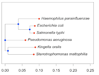
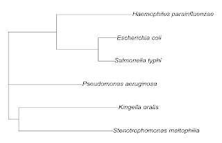
The ta-ta-ta-taa (Melvin video at 2:51) figure is here:


You can compare it with the original plot by the APE package:


And here is the listing for the R code:


ex=c(0.08401,0.08853,0.0595,0.08516,0.0871,0.09976)
ey=c(1.0,2.0,3.0,4.0,5.0,6.0)
ix=c(0.00827,0.07219,0.03863,0.0)
iy=c(1.5,4.5,5.25,3.0)
par(cex=1.5,yaxt='n')
X = max(ex) + 0.15
Y = max(c(max(ey),max(iy))) + 2
plot(ex,ey,xlim=c(0,X),
ylim=c(0,Y),type="n",
xlab='',ylab='')
lines(c(0.00827,0.08401),c(1.0,1.0))
text(0.08401,1.0,label="Stenotrophomonas maltophilia",pos=4,font=3)
lines(c(0.00827,0.08853),c(2.0,2.0))
text(0.08853,2.0,label="Kingella oralis",pos=4,font=3)
lines(c(0.0,0.0595),c(3.0,3.0))
text(0.0595,3.0,label="Pseudomonas aeruginosa",pos=4,font=3)
lines(c(0.07219,0.08516),c(4.0,4.0))
text(0.08516,4.0,label="Salmonella typhi",pos=4,font=3)
lines(c(0.07219,0.0871),c(5.0,5.0))
text(0.0871,5.0,label="Escherichia coli",pos=4,font=3)
lines(c(0.03863,0.09976),c(6.0,6.0))
text(0.09976,6.0,label="Haemophilus parainfluenzae",pos=4,font=3)
lines(c(0.0,0.00827),c(1.5,1.5))
lines(c(0.03863,0.07219),c(4.5,4.5))
lines(c(0.0,0.03863),c(5.25,5.25))
lines(c(0.00827,0.00827),c(1.0,2.0))
lines(c(0.07219,0.07219),c(4.0,5.0))
lines(c(0.03863,0.03863),c(4.5,6.0))
lines(c(0.0,0.0),c(1.5,5.25))
points(ex,ey,pch=16,col="red")
points(ix,iy,pch=16,col="blue")


Phylogenetic Trees: node positions

In this post, we'll continue working with the tree from last time. The data we recovered for the tree looks like this:

external nodes:
E1 Stenotrophomonas_maltophilia 0.07574
E2 Kingella_oralis 0.08026
E3 Pseudomonas_aeruginosa 0.05950
E4 Salmonella_typhi 0.01297
E5 Escherichia_coli 0.01491
E6 Haemophilus_parainfluenzae 0.06113

((E1,E2):0.00827,E3,((E4,E5):0.03356,E6):0.03863);

internal nodes:
I1 E1 E2 0.00827
I2 E4 E5 0.03356
I3 I2 E6 0.03863
I4 I1 E3 I3 0


It's in a file on disk called 'tree.data.txt'. The next step is to load it back into memory and organize it into two dictionaries, one for external and one for internal nodes. We also make a "reverseTree" dictionary where subnodes point to their parents. At the end of the initial phase, we can print the contents to the screen to verify things are OK.


E5 {'dist': '0.01491', 'name': 'Escherichia_coli'}
E4 {'dist': '0.01297', 'name': 'Salmonella_typhi'}
E6 {'dist': '0.06113', 'name': 'Haemophilus_parainfluenzae'}
E1 {'dist': '0.07574', 'name': 'Stenotrophomonas_maltophilia'}
E3 {'dist': '0.05950', 'name': 'Pseudomonas_aeruginosa'}
E2 {'dist': '0.08026', 'name': 'Kingella_oralis'}
-----
I1 {'dist': '0.00827', 'subnodes': ['E1', 'E2']}
I3 {'dist': '0.03863', 'subnodes': ['I2', 'E6']}
I2 {'dist': '0.03356', 'subnodes': ['E4', 'E5']}
I4 {'dist': '0', 'subnodes': ['I1', 'E3', 'I3']}
-----
{'I1': 'I4', 'I3': 'I4', 'I2': 'I3', 'I4': 'root', 'E5': 'I2', 'E4': 'I2', 'E6': 'I3', 'E1': 'I1', 'E3': 'I4', 'E2': 'I1'}


Now, we need to do some work. Each node's x-position will be the sum of all the x-distances back to the root. And the y-position is an integer (1-6) for the external nodes.

For the internal nodes it's a little trickier. The y-position is the average of the y-positions of its subnodes (or the median, if there are three of them). We also need to remember the values for the extreme y-positions of the subnodes (for the vertical bars in the plot). We save these in a separate dictionary called zD.

When we're done, we print out the values for each node to check them over.

We have the node name, parent, x-position and y-position, label (e.g. Escherichia coli), and finally for internal nodes, the min and max of the subnode y positions. Looks good to me.

I1 I4 0.00827 1.5 I1 (1, 2)
I3 I4 0.03863 5.25 I3 (4.5, 6)
I2 I3 0.07219 4.5 I2 (4, 5)
I4 root 0.0 3.0 I4 (1.5, 5.25)
E5 I2 0.0871 5.0 Escherichia_coli
E4 I2 0.08516 4.0 Salmonella_typhi
E6 I3 0.09976 6.0 Haemophilus_parainfluenzae
E1 I1 0.08401 1.0 Stenotrophomonas_maltophilia
E3 I4 0.0595 3.0 Pseudomonas_aeruginosa
E2 I1 0.08853 2.0 Kingella_oralis


Before I started working on this problem earlier in the week, I remembered that I had posted about it before. But I couldn't find my code from the last time, (and I forgot that I'd posted that as well---another senior moment!) Anyway, this solution is much shorter and quite a bit simpler. The complex part is what we did today, working out the x and y positions of each node, as well as (next time) mapping the lines that connecting them, and finally coercing R into doing the plot.

The entire listing:

import sys

def readData(fn):
FH = open(fn)
data = FH.read()
FH.close()
return data.strip()

def loadData():
fn = 'tree.data.txt'
data = readData(fn)
t = data.split('\n\n')
eNodeD = dict()
iNodeD = dict()

L = t[0].split('\n')
for line in L[1:]:
eNode,name,dist = line.strip().split()
eNodeD[eNode] = { 'name':name,'dist':dist }

L = t[2].split('\n')
for line in L[1:]:
t = line.strip().split()
name = t.pop(0)
dist = t.pop()
iNodeD[name] = { 'dist':dist,'subnodes':t }
return eNodeD,iNodeD
#----------------------------------------------
def getReverseTree(eNodeD,iNodeD):
def super(s):
for k in iNodeD:
if s in iNodeD[k]['subnodes']:
return k
return 'root'
rT = dict()
for n in eNodeD: rT[n] = super(n)
for n in iNodeD: rT[n] = super(n)
return rT

def init(v=False):
def report():
for k in eNodeD:
print k, eNodeD[k]
print '-----'
for k in iNodeD:
print k, iNodeD[k]
print '-----'
print rT
eNodeD,iNodeD = loadData()
rT = getReverseTree(eNodeD,iNodeD)
if v: report()
return eNodeD,iNodeD,rT
#------------------------------------
def doPositions(eNodeD,iNodeD,rT):
# x pos are distance from root
xD = dict()
for k in eNodeD.keys() + iNodeD.keys():
if k in eNodeD:
x = float(eNodeD[k]['dist'])
else:
x = float(iNodeD[k]['dist'])
super = rT[k]
while super is not 'root':
x += float(iNodeD[super]['dist'])
super = rT[super]
xD[k] = x

# y pos for eNodes are numbered sequentially
yD = dict()
for i,k in enumerate(sorted(eNodeD.keys())):
yD[k] = i+1

# for internal nodes:
# y = average of y of direct descendants
# or the median
# must also keep extreme y's for lines
zD = dict()

for k in sorted(iNodeD.keys()):
L = iNodeD[k]['subnodes']
L = [yD[n] for n in L]
if len(L) == 3:
yD[k] = L[1]
else:
yD[k] = sum(L)*1.0/len(L)
zD[k] = min(L),max(L)
return xD,yD,zD
#----------------------------------------------
# see what we got
def second_report(xD,yD,zD,eNodeD,rT):
for k in xD:
print k, rT[k],
print round(xD[k],5),
print round(yD[k],2),
if k in eNodeD:
print eNodeD[k]['name']
else:
print k,
print zD[k]
#----------------------------------------------
if __name__ == '__main__':
eNodeD,iNodeD,rT = init(v=True)
xD,yD,zD = doPositions(eNodeD,iNodeD,rT)
second_report(xD,yD,zD,eNodeD,rT)

Phylogenetic Trees: parsing

Continuing toward the goal of being able to manipulate (and print) phylogenetic trees, I wrote a simple parser for the Newick format.

(Note: This has not been tested very much, although it does work on several examples that I tried. It is just a toy program for use in exploring what trees are about).

The parser works in three phases:

First, we process each character of the input and recognize the five special characters '():,;', generating a list of tokens. Disregarding newlines and other characters that are not valid, we accumulate standard characters in a buffer which is flushed when a special character is encountered.

Here is the first 7 lines of the output for the tree from last time:

(
(
Stenotrophomonas_maltophilia
:
0.07574
,
Kingella_oralis


In phase two, we make note of names and distances from each external node to its parental (internal) node. The external node information in the tree is replaced by a short name. Here is the output of the second stage:

external nodes:
E1 Stenotrophomonas_maltophilia 0.07574
E2 Kingella_oralis 0.08026
E3 Pseudomonas_aeruginosa 0.05950
E4 Salmonella_typhi 0.01297
E5 Escherichia_coli 0.01491
E6 Haemophilus_parainfluenzae 0.06113


The tree after this step:

((E1,E2):0.00827,E3,((E4,E5):0.03356,E6):0.03863);


(There is a trick in the second step. Because we are modifying the list of tree elements within this function, we process the external nodes in reverse order. This ensures that all the other indexes remain valid).

In the third and final phase, we break down the structure of the tree into its internal nodes. Each internal node gets a name, a list of its sub-nodes, and the distance to its parental node. The output is shown below. The information for the external and internal nodes will be written as text to disk and then processed further.

internal nodes:
I1 E1 E2 0.00827
I2 E4 E5 0.03356
I3 I2 E6 0.03863
I4 I1 E3 I3 0


After processing the first two internal nodes, the tree looks like this:

(I1,E3,(I2,E6):0.03863);


The full listing:

UC = 'ABCDEFGHIJKLMNOPQRSTUVWXYZ'
LC = UC.lower()
digits = '0123456789'
punc = '._- '
chars = UC + LC + digits + punc
special = '():,;'

def loadData(fn):
FH = open(fn)
data = FH.read().strip()
FH.close()
return data

def parseData(s):
rL = list()
temp = list()
for c in s:
if c in chars:
temp.append(c)
elif c in special:
if temp:
rL.append(''.join(temp))
temp = list()
rL.append(c)
return rL
#-------------------------------------------
def doExternalNodes(L):
iL = list()
eNodeL = list()
# get pos for ':' for external nodes
for i,e in enumerate(L):
if e == ':':
# internal nodes have '):'
if not L[i-1] == ')':
iL.append(i)
eNodeCount = len(iL)
# reverse to keep indexes valid below
for i in reversed(iL):
name = L[i-1]
dist = L[i+1]
n = 'E' + str(eNodeCount)
eNodeCount -= 1
eNodeL.append((n,name,dist))
# replace the node with n
L = L[:i-1] + [n] + L[i+2:]
return L, reversed(eNodeL)
#-------------------------------------------
def findInternalNode(L):
# every ')' comes at the end of an iNode
try: j = L.index(')')
except ValueError: return None
i = j
while L[i] != '(': i -= 1
return i,j

def doInternalNodes(L):
iNodeCount = 0
iNodeL = list()
t = findInternalNode(L)
while t:
i,j = t
j += 2 # move out to dist
iNodeCount += 1
n = 'I' + str(iNodeCount)
# root may not have a dist
try:
dist = L[j]
except IndexError:
dist = 0
assert L[j-1] == ';'
# may have more than two sub-nodes:
nodes = list()
for k in range(i+1,j-2,2):
#print k, L[k]
nodes.append(L[k])
iNodeL.append((n,nodes,dist))
L = L[:i] + [n] + L[j+1:]
t = findInternalNode(L)
return L, iNodeL
#-------------------------------------------
data = loadData(fn = 'seq.phy.txt')
L = parseData(data)
#for e in L: print e
#print
#-------------------------------------------
L,eNodeL = doExternalNodes(L)
print 'external nodes:'
for e in eNodeL:
print e[0],e[1],e[2]
print
print ''.join(L) + '\n'
#-------------------------------------------
L,iNodeL = doInternalNodes(L)
print 'internal nodes:'
for e in iNodeL:
print e[0],
for n in e[1]: print n,
print e[2]