Calculus in 5 minutes (part 3)

This is a series about the essence, the merest whiff of the perfume of calculus. The first and second posts are here and here. Differentiation is useful, but integration allows us to do things which are nothing short of miraculous. For example, consider this modestly complex equation, and its curve.

y = x3 - x2 - x + 150

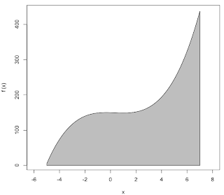
The integral calculus (the second part) allows us to easily calculate the area under this curve (between the curve and the x-axis), as shown in gray.

Remember what we said before: the relationship between the function which we plot as a curve, and its slope at any point is found by differentiating f(x) to f '(x). The slope is f '(x). The secret of integral calculus (don't tell anybody) is that the same relationship holds between the area under a curve, and the curve itself, but in reverse. That is, if the curve is f '(x), the area is f(x). It's that simple.

If we know f '(x), how do we find f(x)? Sometimes it's easy and sometimes it's hard. Suppose that every time we have a function f(x) and we find f '(x), we write the result down and save it in our little black book. When we encounter a function in an integration problem, we look in the book.

For the example, we need a function f(x), which when differentiated gives:

y' = x3 - x2 - x + 150

We look in our book, and there it is:

y = x4/4 - x3/3 - x2/2 + 150 x

Of course, the area depends on which endpoints we choose. (Looking at the figure should make this clear). So evaluate the integrated function between the limits x = 7 and x = -5. We have:

74/4 - 73/3 - 72/2 + 7*150 minus (-5)4/4 - (-5)3/3 - (-5)2/2 + (-5)*150

I get:

2401/4 - 343/3 - 49/2 + 1050 - 625/4 + 125/3 - 25/2 - 750

I'm too lazy to finish it. But I'll check the method itself by an interesting approach in the next post.

Why do I say it's a miracle? Because we get the area from the integrated equation just by using the endpoints. We don't have to worry about what lies between. That is amazing.

R code: f <- function(x) { return (x**3 - x**2 - x + 150) } plot (f,-5,7,xlim=c(-6,8),cex=3) xvals = seq(-5,7,length=1000) yvals = f(xvals) x = c(xvals,rev(xvals)) y = c(rep(0,1000),rev(yvals)) polygon(x,y,col='gray')